

9 Accelerator Operations
539
The Fast Fourier Transform (FFT) of the BPM signal, z(N), offers a poor
resolution on the phase measurement. Interpolated FTs like [28] or Singular Value
Decomposition (SVD) algorithms like [29] feature a higher performance in terms of
spectral resolution. The achievable resolution is usually limited by decoherence processes that damp the bunch centroid oscillations. Furthermore, beam decoherence
also affects FT amplitudes and phases, which can be partially restored [30, 31, 42].
These limitations can be overcome by forcing betatron oscillations with the aid of
an AC dipole with a frequency close to the machine tune. Moreover, if the AC dipole
is ramped up and down adiabatically the beam emittance is preserved [32, 33].
The beam dynamics with forced oscillations features remarkable differences
from that of free oscillations [34–37]. In presence of an AC dipole the measured
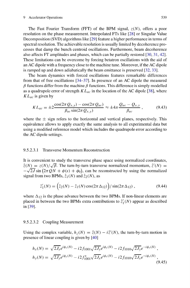
β functions differ from the machine β functions. This difference is simply modelled
as a quadrupole error of strength KL ac in the location of the AC dipole [38], where
KL ac is given by
KL ac = ±2
cos(2πQ x,y ) − cos(2πQ ac )
β ac sin(2πQ x,y )
≈ ±4π
Q ac − Q x,y
β ac
,
(9.43)
where the ± sign refers to the horizontal and vertical planes, respectively. This
equivalence allows to apply exactly the same analysis to all experimental data but
using a modified reference model which includes the quadrupole error according to
the AC dipole settings.
9.5.2.3.1 Transverse Momentum Reconstruction
It is convenient to study the transverse phase space using normalized coordinates,
ˆ
z(N) = z(N)/
√
β. The turn-by-turn transverse normalized momentum, ˆ
z (N) =
−
√
2J sin
2πQN + φ(s) + φ 0
, can be reconstructed by using the normalized
signal from two BPMs, ˆ
z 1 (N) and ˆ
z 2 (N), as
ˆ
z
1 (N) =
ˆ
z 2 (N) − ˆ
z 1 (N) cos(2ππ 12 )
/ sin(2ππ 12 ) ,
(9.44)
where 12 is the phase advance between the two BPMs. If non-linear elements are
placed in between the two BPMs extra contributions to ˆ
z
1 (N) appear as described
in [39].
9.5.2.3.2 Coupling Measurement
Using the complex variable, h z (N) = ˆ
z(N) − i ˆ
z (N), the turn-by-turn motion in
presence of linear coupling is given by [40]
h x (N) =
2J x e
iφ x (N)
− i2f 1001
2J y e
iφ y (N)
− i2f 1010
2J y e
−iφ y (N) ,
h y (N) =
2J y e
iφ y (N)
− i2f
∗
1001
2J x e
iφ x (N)
− i2f 1010
2J x e
−iφ x (N) ,
(9.45)
539
The Fast Fourier Transform (FFT) of the BPM signal, z(N), offers a poor
resolution on the phase measurement. Interpolated FTs like [28] or Singular Value
Decomposition (SVD) algorithms like [29] feature a higher performance in terms of
spectral resolution. The achievable resolution is usually limited by decoherence processes that damp the bunch centroid oscillations. Furthermore, beam decoherence
also affects FT amplitudes and phases, which can be partially restored [30, 31, 42].
These limitations can be overcome by forcing betatron oscillations with the aid of
an AC dipole with a frequency close to the machine tune. Moreover, if the AC dipole
is ramped up and down adiabatically the beam emittance is preserved [32, 33].
The beam dynamics with forced oscillations features remarkable differences
from that of free oscillations [34–37]. In presence of an AC dipole the measured
β functions differ from the machine β functions. This difference is simply modelled
as a quadrupole error of strength KL ac in the location of the AC dipole [38], where
KL ac is given by
KL ac = ±2
cos(2πQ x,y ) − cos(2πQ ac )
β ac sin(2πQ x,y )
≈ ±4π
Q ac − Q x,y
β ac
,
(9.43)
where the ± sign refers to the horizontal and vertical planes, respectively. This
equivalence allows to apply exactly the same analysis to all experimental data but
using a modified reference model which includes the quadrupole error according to
the AC dipole settings.
9.5.2.3.1 Transverse Momentum Reconstruction
It is convenient to study the transverse phase space using normalized coordinates,
ˆ
z(N) = z(N)/
√
β. The turn-by-turn transverse normalized momentum, ˆ
z (N) =
−
√
2J sin
2πQN + φ(s) + φ 0
, can be reconstructed by using the normalized
signal from two BPMs, ˆ
z 1 (N) and ˆ
z 2 (N), as
ˆ
z
1 (N) =
ˆ
z 2 (N) − ˆ
z 1 (N) cos(2ππ 12 )
/ sin(2ππ 12 ) ,
(9.44)
where 12 is the phase advance between the two BPMs. If non-linear elements are
placed in between the two BPMs extra contributions to ˆ
z
1 (N) appear as described
in [39].
9.5.2.3.2 Coupling Measurement
Using the complex variable, h z (N) = ˆ
z(N) − i ˆ
z (N), the turn-by-turn motion in
presence of linear coupling is given by [40]
h x (N) =
2J x e
iφ x (N)
− i2f 1001
2J y e
iφ y (N)
− i2f 1010
2J y e
−iφ y (N) ,
h y (N) =
2J y e
iφ y (N)
− i2f
∗
1001
2J x e
iφ x (N)
− i2f 1010
2J x e
−iφ x (N) ,
(9.45)