

9 Accelerator Operations
531
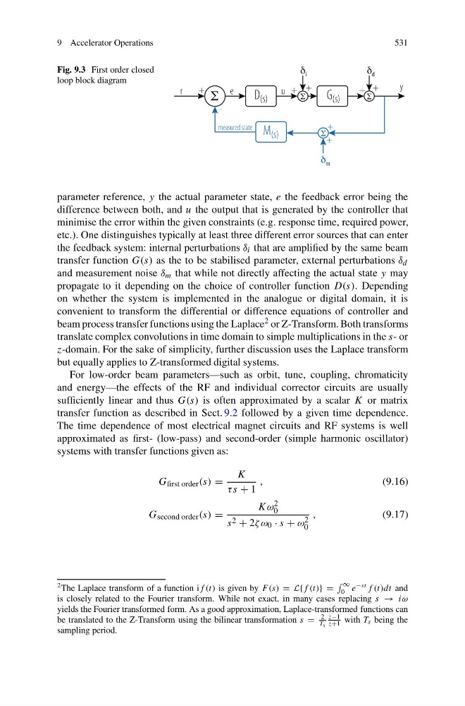
Fig. 9.3 First order closed
loop block diagram
D (s)
M (s)
measured state
G (s)
r
e
u
i
d
m
+
+
+
+
+
y
+
+
–
parameter reference, y the actual parameter state, e the feedback error being the
difference between both, and u the output that is generated by the controller that
minimise the error within the given constraints (e.g. response time, required power,
etc.). One distinguishes typically at least three different error sources that can enter
the feedback system: internal perturbations δ i that are amplified by the same beam
transfer function G(s) as the to be stabilised parameter, external perturbations δ d
and measurement noise δ m that while not directly affecting the actual state y may
propagate to it depending on the choice of controller function D(s). Depending
on whether the system is implemented in the analogue or digital domain, it is
convenient to transform the differential or difference equations of controller and
beam process transfer functions using the Laplace 2 or Z-Transform. Both transforms
translate complex convolutions in time domain to simple multiplications in the s- or
z-domain. For the sake of simplicity, further discussion uses the Laplace transform
but equally applies to Z-transformed digital systems.
For low-order beam parameters—such as orbit, tune, coupling, chromaticity
and energy—the effects of the RF and individual corrector circuits are usually
sufficiently linear and thus G(s) is often approximated by a scalar K or matrix
transfer function as described in Sect. 9.2 followed by a given time dependence.
The time dependence of most electrical magnet circuits and RF systems is well
approximated as first- (low-pass) and second-order (simple harmonic oscillator)
systems with transfer functions given as:
G first order (s) =
K
τ s + 1
,
(9.16)
G second order (s) =
Kω 2
0
s 2 + 2ζ ω 0 · s + ω 2
0
,
(9.17)
2 The Laplace transform of a function if (t) is given by F (s) = L{f (t)} =
∞
0 e −st f (t)dt and
is closely related to the Fourier transform. While not exact, in many cases replacing s → iω
yields the Fourier transformed form. As a good approximation, Laplace-transformed functions can
be translated to the Z-Transform using the bilinear transformation s =
2
Ts
z−1
z+1 with T s being the
sampling period.
531
Fig. 9.3 First order closed
loop block diagram
D (s)
M (s)
measured state
G (s)
r
e
u
i
d
m
+
+
+
+
+
y
+
+
–
parameter reference, y the actual parameter state, e the feedback error being the
difference between both, and u the output that is generated by the controller that
minimise the error within the given constraints (e.g. response time, required power,
etc.). One distinguishes typically at least three different error sources that can enter
the feedback system: internal perturbations δ i that are amplified by the same beam
transfer function G(s) as the to be stabilised parameter, external perturbations δ d
and measurement noise δ m that while not directly affecting the actual state y may
propagate to it depending on the choice of controller function D(s). Depending
on whether the system is implemented in the analogue or digital domain, it is
convenient to transform the differential or difference equations of controller and
beam process transfer functions using the Laplace 2 or Z-Transform. Both transforms
translate complex convolutions in time domain to simple multiplications in the s- or
z-domain. For the sake of simplicity, further discussion uses the Laplace transform
but equally applies to Z-transformed digital systems.
For low-order beam parameters—such as orbit, tune, coupling, chromaticity
and energy—the effects of the RF and individual corrector circuits are usually
sufficiently linear and thus G(s) is often approximated by a scalar K or matrix
transfer function as described in Sect. 9.2 followed by a given time dependence.
The time dependence of most electrical magnet circuits and RF systems is well
approximated as first- (low-pass) and second-order (simple harmonic oscillator)
systems with transfer functions given as:
G first order (s) =
K
τ s + 1
,
(9.16)
G second order (s) =
Kω 2
0
s 2 + 2ζ ω 0 · s + ω 2
0
,
(9.17)
2 The Laplace transform of a function if (t) is given by F (s) = L{f (t)} =
∞
0 e −st f (t)dt and
is closely related to the Fourier transform. While not exact, in many cases replacing s → iω
yields the Fourier transformed form. As a good approximation, Laplace-transformed functions can
be translated to the Z-Transform using the bilinear transformation s =
2
Ts
z−1
z+1 with T s being the
sampling period.