

526
M. Lamont et al.
From Eq.(9.7), it follows that (α = 1, . . . , N),
A v
(α)
= w α
u
(α) , A
t
u
(α)
= w α
v
(α) ,
(9.8)
and
AA
t
u
(α)
= w
2
α
u
(α) , A
t A v
(α)
= w
2
α
v
(α) .
(9.9)
When none of the diagonal elements w α vanish, the solution of Eq.(9.5) is
θ =
−VW
−1 U t
d.
d may be expanded in terms of eigenvectors
u (α) [4],
d =
N
α=1
C α
u
(α)
+
d 0 ,
(9.10)
where C α =
d · ·
u (α) , while
d 0 corresponds to the uncorrectable part of the orbit.
The corrector strength required for correction is
θ = −
N
α=1
C α
w α
v
(α) .
(9.11)
If a given w α = 0 indicating that the matrix is singular, one discards the
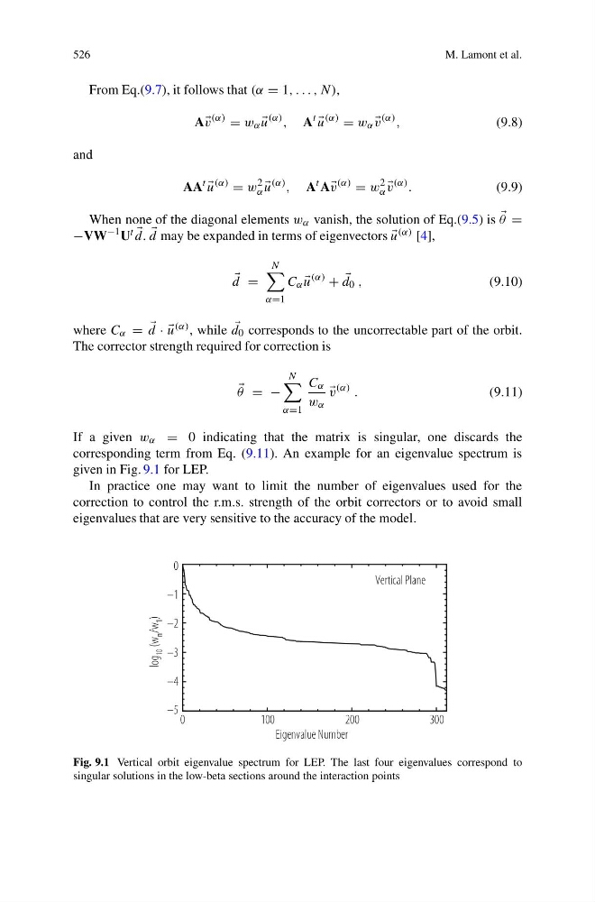
corresponding term from Eq. (9.11). An example for an eigenvalue spectrum is
given in Fig. 9.1 for LEP.
In practice one may want to limit the number of eigenvalues used for the
correction to control the r.m.s. strength of the orbit correctors or to avoid small
eigenvalues that are very sensitive to the accuracy of the model.
Eigenvalue Number
Vertical Plane
–5
–4
–3
–2
–1
0
0
100
200
300
log
10 (w
n /w
1 )
Fig. 9.1 Vertical orbit eigenvalue spectrum for LEP. The last four eigenvalues correspond to
singular solutions in the low-beta sections around the interaction points
M. Lamont et al.
From Eq.(9.7), it follows that (α = 1, . . . , N),
A v
(α)
= w α
u
(α) , A
t
u
(α)
= w α
v
(α) ,
(9.8)
and
AA
t
u
(α)
= w
2
α
u
(α) , A
t A v
(α)
= w
2
α
v
(α) .
(9.9)
When none of the diagonal elements w α vanish, the solution of Eq.(9.5) is
θ =
−VW
−1 U t
d.
d may be expanded in terms of eigenvectors
u (α) [4],
d =
N
α=1
C α
u
(α)
+
d 0 ,
(9.10)
where C α =
d · ·
u (α) , while
d 0 corresponds to the uncorrectable part of the orbit.
The corrector strength required for correction is
θ = −
N
α=1
C α
w α
v
(α) .
(9.11)
If a given w α = 0 indicating that the matrix is singular, one discards the
corresponding term from Eq. (9.11). An example for an eigenvalue spectrum is
given in Fig. 9.1 for LEP.
In practice one may want to limit the number of eigenvalues used for the
correction to control the r.m.s. strength of the orbit correctors or to avoid small
eigenvalues that are very sensitive to the accuracy of the model.
Eigenvalue Number
Vertical Plane
–5
–4
–3
–2
–1
0
0
100
200
300
log
10 (w
n /w
1 )
Fig. 9.1 Vertical orbit eigenvalue spectrum for LEP. The last four eigenvalues correspond to
singular solutions in the low-beta sections around the interaction points