

4 Impedance and Collective Effects
153
limit
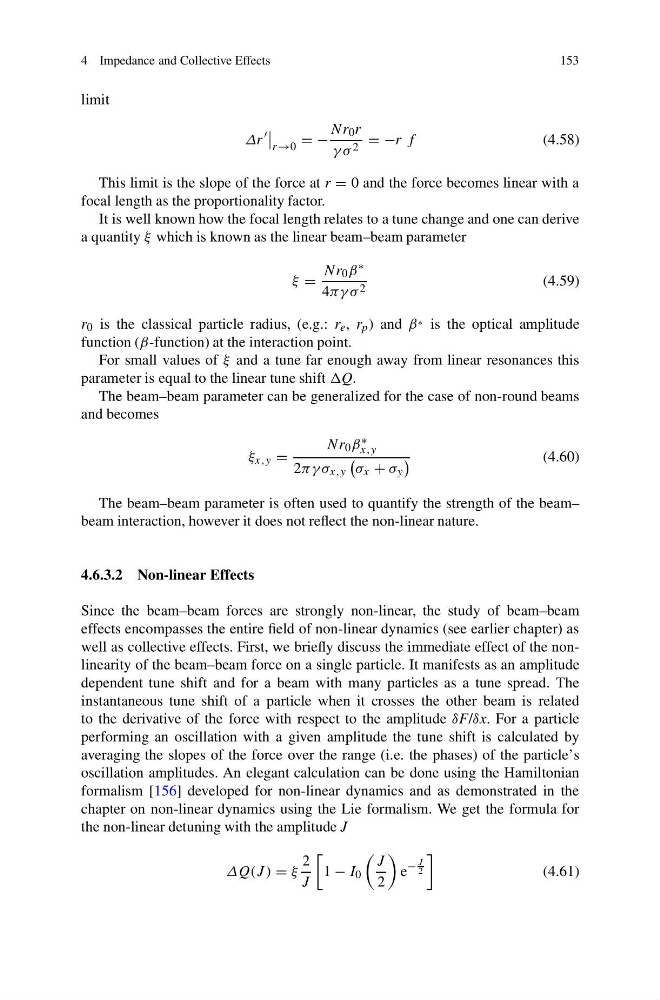
Δr
r→0
= −
Nr 0 r
γ σ 2 = −r f
(4.58)
This limit is the slope of the force at r = 0 and the force becomes linear with a
focal length as the proportionality factor.
It is well known how the focal length relates to a tune change and one can derive
a quantity ξ which is known as the linear beam–beam parameter
ξ =
Nr 0 β ∗
4πγ σ 2
(4.59)
r 0 is the classical particle radius, (e.g.: r e , r p ) and β ∗ is the optical amplitude
function (β-function) at the interaction point.
For small values of ξ and a tune far enough away from linear resonances this
parameter is equal to the linear tune shift
The beam–beam parameter can be generalized for the case of non-round beams
and becomes
ξ x,y =
Nr 0 β ∗
x,y
2πγ σ x,y
σ x + σ y
(4.60)
The beam–beam parameter is often used to quantify the strength of the beam–
beam interaction, however it does not reflect the non-linear nature.
4.6.3.2 Non-linear Effects
Since the beam–beam forces are strongly non-linear, the study of beam–beam
effects encompasses the entire field of non-linear dynamics (see earlier chapter) as
well as collective effects. First, we briefly discuss the immediate effect of the nonlinearity of the beam–beam force on a single particle. It manifests as an amplitude
dependent tune shift and for a beam with many particles as a tune spread. The
instantaneous tune shift of a particle when it crosses the other beam is related
to the derivative of the force with respect to the amplitude δF/δx. For a particle
performing an oscillation with a given amplitude the tune shift is calculated by
averaging the slopes of the force over the range (i.e. the phases) of the particle’s
oscillation amplitudes. An elegant calculation can be done using the Hamiltonian
formalism [156] developed for non-linear dynamics and as demonstrated in the
chapter on non-linear dynamics using the Lie formalism. We get the formula for
the non-linear detuning with the amplitude J
ΔQ(J ) = ξ
2
J
1 − I 0
J
2
e
−
J
2
(4.61)
153
limit
Δr
r→0
= −
Nr 0 r
γ σ 2 = −r f
(4.58)
This limit is the slope of the force at r = 0 and the force becomes linear with a
focal length as the proportionality factor.
It is well known how the focal length relates to a tune change and one can derive
a quantity ξ which is known as the linear beam–beam parameter
ξ =
Nr 0 β ∗
4πγ σ 2
(4.59)
r 0 is the classical particle radius, (e.g.: r e , r p ) and β ∗ is the optical amplitude
function (β-function) at the interaction point.
For small values of ξ and a tune far enough away from linear resonances this
parameter is equal to the linear tune shift
The beam–beam parameter can be generalized for the case of non-round beams
and becomes
ξ x,y =
Nr 0 β ∗
x,y
2πγ σ x,y
σ x + σ y
(4.60)
The beam–beam parameter is often used to quantify the strength of the beam–
beam interaction, however it does not reflect the non-linear nature.
4.6.3.2 Non-linear Effects
Since the beam–beam forces are strongly non-linear, the study of beam–beam
effects encompasses the entire field of non-linear dynamics (see earlier chapter) as
well as collective effects. First, we briefly discuss the immediate effect of the nonlinearity of the beam–beam force on a single particle. It manifests as an amplitude
dependent tune shift and for a beam with many particles as a tune spread. The
instantaneous tune shift of a particle when it crosses the other beam is related
to the derivative of the force with respect to the amplitude δF/δx. For a particle
performing an oscillation with a given amplitude the tune shift is calculated by
averaging the slopes of the force over the range (i.e. the phases) of the particle’s
oscillation amplitudes. An elegant calculation can be done using the Hamiltonian
formalism [156] developed for non-linear dynamics and as demonstrated in the
chapter on non-linear dynamics using the Lie formalism. We get the formula for
the non-linear detuning with the amplitude J
ΔQ(J ) = ξ
2
J
1 − I 0
J
2
e
−
J
2
(4.61)