

4 Impedance and Collective Effects
151
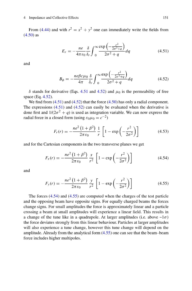
From (4.44) and with r 2 = x 2 + y 2 one can immediately write the fields from
(4.50) as
E r = −
ne
4πε 0
δ
δ r
∞
0
exp
−
r 2
2σ 2 +q
2σ 2 + q
dq
(4.51)
and
B φ = −
neβcμ 0
4π
δ
δ r
∞
0
exp
−
r 2
2σ 2 +q
2σ 2 + q
dq
(4.52)
δ stands for derivative (Eqs. 4.51 and 4.52) and μ 0 is the permeability of free
space (Eq. 4.52).
We find from (4.51) and (4.52) that the force (4.50) has only a radial component.
The expressions (4.51) and (4.52) can easily be evaluated when the derivative is
done first and 1/(2σ 2 + q) is used as integration variable. We can now express the
radial force in a closed form (using ε 0 μ 0 = c −2 )
F r (r) = −
ne 2
1 + β 2
2πε 0
1
r
1 − exp
−
r 2
2σ 2
(4.53)
and for the Cartesian components in the two transverse planes we get
F x (r) = −
ne 2
1 + β 2
2πε 0
x
r 2
1 − exp
−
r 2
2σ 2
(4.54)
and
F y (r) = −
ne 2
1 + β 2
2πε 0
y
r 2
1 − exp
−
r 2
2σ 2
(4.55)
The forces (4.54) and (4.55) are computed when the charges of the test particle
and the opposing beam have opposite signs. For equally charged beams the forces
change signs. For small amplitudes the force is approximately linear and a particle
crossing a beam at small amplitudes will experience a linear field. This results in
a change of the tune like in a quadrupole. At larger amplitudes (i.e. above ~1σ )
the force deviates strongly from this linear behaviour. Particles at larger amplitudes
will also experience a tune change, however this tune change will depend on the
amplitude. Already from the analytical form (4.55) one can see that the beam–beam
force includes higher multipoles.
151
From (4.44) and with r 2 = x 2 + y 2 one can immediately write the fields from
(4.50) as
E r = −
ne
4πε 0
δ
δ r
∞
0
exp
−
r 2
2σ 2 +q
2σ 2 + q
dq
(4.51)
and
B φ = −
neβcμ 0
4π
δ
δ r
∞
0
exp
−
r 2
2σ 2 +q
2σ 2 + q
dq
(4.52)
δ stands for derivative (Eqs. 4.51 and 4.52) and μ 0 is the permeability of free
space (Eq. 4.52).
We find from (4.51) and (4.52) that the force (4.50) has only a radial component.
The expressions (4.51) and (4.52) can easily be evaluated when the derivative is
done first and 1/(2σ 2 + q) is used as integration variable. We can now express the
radial force in a closed form (using ε 0 μ 0 = c −2 )
F r (r) = −
ne 2
1 + β 2
2πε 0
1
r
1 − exp
−
r 2
2σ 2
(4.53)
and for the Cartesian components in the two transverse planes we get
F x (r) = −
ne 2
1 + β 2
2πε 0
x
r 2
1 − exp
−
r 2
2σ 2
(4.54)
and
F y (r) = −
ne 2
1 + β 2
2πε 0
y
r 2
1 − exp
−
r 2
2σ 2
(4.55)
The forces (4.54) and (4.55) are computed when the charges of the test particle
and the opposing beam have opposite signs. For equally charged beams the forces
change signs. For small amplitudes the force is approximately linear and a particle
crossing a beam at small amplitudes will experience a linear field. This results in
a change of the tune like in a quadrupole. At larger amplitudes (i.e. above ~1σ )
the force deviates strongly from this linear behaviour. Particles at larger amplitudes
will also experience a tune change, however this tune change will depend on the
amplitude. Already from the analytical form (4.55) one can see that the beam–beam
force includes higher multipoles.