

150
E. Metral et al.
4.6.2.1 Elliptical Beams
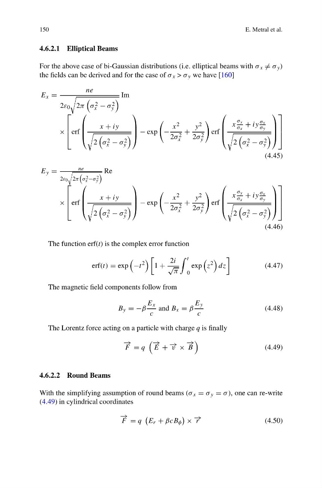
For the above case of bi-Gaussian distributions (i.e. elliptical beams with σ x = σ y )
the fields can be derived and for the case of σ x > σ y we have [160]
E x =
ne
2ε 0
2π
σ 2
x − σ 2
y
Im
×
⎡
⎢
⎢
⎣ erf
⎛
⎜
⎜
⎝
x + iy
2
σ 2
x − σ 2
y
⎞
⎟
⎟
⎠ − exp
−
x 2
2σ 2
x
+
y 2
2σ 2
y
erf
⎛
⎜
⎜
⎝
x
σ y
σ x
+ iy
σ x
σ y
2
σ 2
x − σ 2
y
⎞
⎟
⎟
⎠
⎤
⎥
⎥
⎦
(4.45)
E y =
ne
2ε 0
2π
σ 2
x −σ 2
y
Re
×
⎡
⎢
⎢
⎣ erf
⎛
⎜
⎜
⎝
x + iy
2
σ 2
x − σ 2
y
⎞
⎟
⎟
⎠ − exp
−
x 2
2σ 2
x
+
y 2
2σ 2
y
erf
⎛
⎜
⎜
⎝
x
σ y
σ x
+ iy
σ x
σ y
2
σ 2
x − σ 2
y
⎞
⎟
⎟
⎠
⎤
⎥
⎥
⎦
(4.46)
The function erf(t) is the complex error function
erf(t) = exp
−t
2
1 +
2i
√
π
t
0
exp
z
2
dz
(4.47)
The magnetic field components follow from
B y = −β
E x
c
and B x = β
E y
c
(4.48)
The Lorentz force acting on a particle with charge q is finally
− →
F = q
− →
E + − → v ×
− →
B
(4.49)
4.6.2.2 Round Beams
With the simplifying assumption of round beams (σ x = σ y = σ ), one can re-write
(4.49) in cylindrical coordinates
− →
F = q
E r + βcB φ
× − → r
(4.50)
E. Metral et al.
4.6.2.1 Elliptical Beams
For the above case of bi-Gaussian distributions (i.e. elliptical beams with σ x = σ y )
the fields can be derived and for the case of σ x > σ y we have [160]
E x =
ne
2ε 0
2π
σ 2
x − σ 2
y
Im
×
⎡
⎢
⎢
⎣ erf
⎛
⎜
⎜
⎝
x + iy
2
σ 2
x − σ 2
y
⎞
⎟
⎟
⎠ − exp
−
x 2
2σ 2
x
+
y 2
2σ 2
y
erf
⎛
⎜
⎜
⎝
x
σ y
σ x
+ iy
σ x
σ y
2
σ 2
x − σ 2
y
⎞
⎟
⎟
⎠
⎤
⎥
⎥
⎦
(4.45)
E y =
ne
2ε 0
2π
σ 2
x −σ 2
y
Re
×
⎡
⎢
⎢
⎣ erf
⎛
⎜
⎜
⎝
x + iy
2
σ 2
x − σ 2
y
⎞
⎟
⎟
⎠ − exp
−
x 2
2σ 2
x
+
y 2
2σ 2
y
erf
⎛
⎜
⎜
⎝
x
σ y
σ x
+ iy
σ x
σ y
2
σ 2
x − σ 2
y
⎞
⎟
⎟
⎠
⎤
⎥
⎥
⎦
(4.46)
The function erf(t) is the complex error function
erf(t) = exp
−t
2
1 +
2i
√
π
t
0
exp
z
2
dz
(4.47)
The magnetic field components follow from
B y = −β
E x
c
and B x = β
E y
c
(4.48)
The Lorentz force acting on a particle with charge q is finally
− →
F = q
− →
E + − → v ×
− →
B
(4.49)
4.6.2.2 Round Beams
With the simplifying assumption of round beams (σ x = σ y = σ ), one can re-write
(4.49) in cylindrical coordinates
− →
F = q
E r + βcB φ
× − → r
(4.50)