

4 Impedance and Collective Effects
149
beam effects and in general a self-consistent treatment is required. Although
we now have a good qualitative understanding of the various phenomena, a
complete theory does not exist and exact predictions are still difficult. Numerical
techniques such as computer simulations have been used with great success to
improve the picture on some aspects of the beam–beam interaction while for other
problems the available models are not fully satisfactory in their predictive power
[154].
4.6.2 Beam–Beam Force
In the rest frame of a beam we have only electrostatic fields and to find the forces
on other moving charges, we have to transform the fields into the moving frame and
to calculate the Lorentz forces (see [153, 155–160] and references therein).
The fields are obtained by integrating over the charge distributions. The forces
can be defocusing or focusing since the test particle can have the same or opposite
charge with respect to the beam producing the forces.
The distribution of particles producing the fields can follow various functions,
leading to different fields and forces. It is not always possible to integrate the
distribution to arrive at an analytical expression for the forces in which case either
an approximation or numerical methods have to be used. This is in particular true
for hadron beams, which usually do not experience significant synchrotron radiation
and damping. For e − e + colliders the distribution functions are most likely Gaussian
with truncated tails.
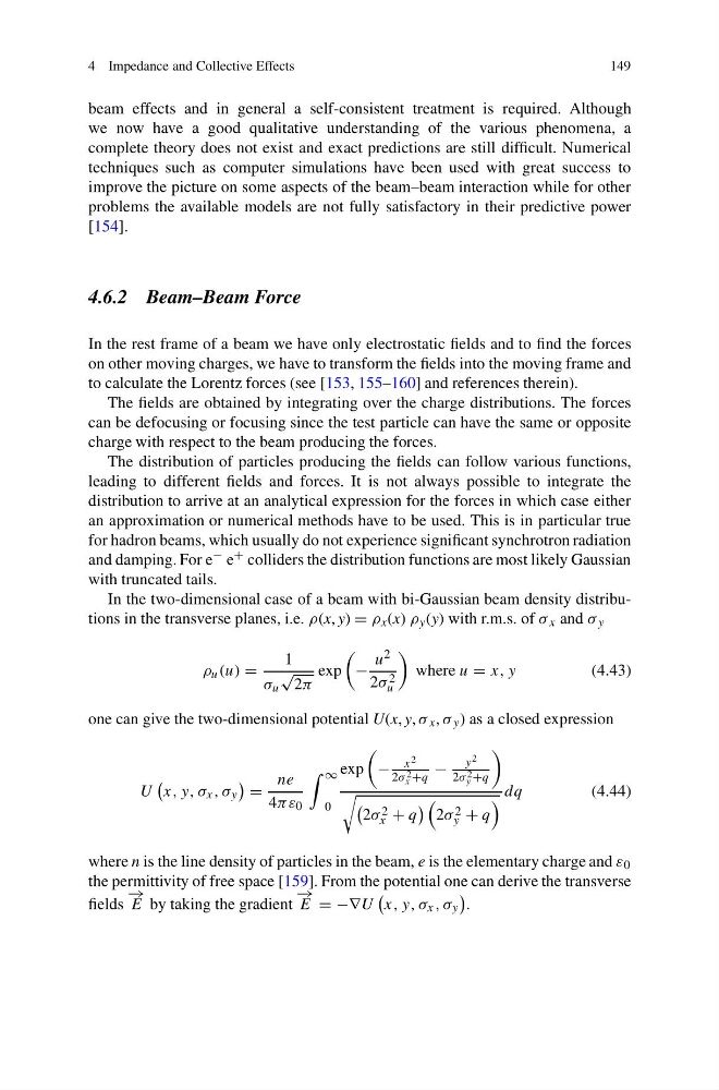
In the two-dimensional case of a beam with bi-Gaussian beam density distributions in the transverse planes, i.e. ρ(x, y) = ρ x (x) ρ y (y) with r.m.s. of σ x and σ y
ρ u (u) =
1
σ u
√
2π
exp
−
u 2
2σ 2
u
where u = x, y
(4.43)
one can give the two-dimensional potential U(x, y, σ x , σ y ) as a closed expression
U
x, y, σ x , σ y
=
ne
4πε 0
∞
0
exp
−
x 2
2σ 2
x +q
−
y 2
2σ 2
y +q
2σ 2
x + q
2σ 2
y + q
dq
(4.44)
where n is the line density of particles in the beam, e is the elementary charge and ε 0
the permittivity of free space [159]. From the potential one can derive the transverse
fields
− →
E by taking the gradient
− →
E = −∇U
x, y, σ x , σ y
.
149
beam effects and in general a self-consistent treatment is required. Although
we now have a good qualitative understanding of the various phenomena, a
complete theory does not exist and exact predictions are still difficult. Numerical
techniques such as computer simulations have been used with great success to
improve the picture on some aspects of the beam–beam interaction while for other
problems the available models are not fully satisfactory in their predictive power
[154].
4.6.2 Beam–Beam Force
In the rest frame of a beam we have only electrostatic fields and to find the forces
on other moving charges, we have to transform the fields into the moving frame and
to calculate the Lorentz forces (see [153, 155–160] and references therein).
The fields are obtained by integrating over the charge distributions. The forces
can be defocusing or focusing since the test particle can have the same or opposite
charge with respect to the beam producing the forces.
The distribution of particles producing the fields can follow various functions,
leading to different fields and forces. It is not always possible to integrate the
distribution to arrive at an analytical expression for the forces in which case either
an approximation or numerical methods have to be used. This is in particular true
for hadron beams, which usually do not experience significant synchrotron radiation
and damping. For e − e + colliders the distribution functions are most likely Gaussian
with truncated tails.
In the two-dimensional case of a beam with bi-Gaussian beam density distributions in the transverse planes, i.e. ρ(x, y) = ρ x (x) ρ y (y) with r.m.s. of σ x and σ y
ρ u (u) =
1
σ u
√
2π
exp
−
u 2
2σ 2
u
where u = x, y
(4.43)
one can give the two-dimensional potential U(x, y, σ x , σ y ) as a closed expression
U
x, y, σ x , σ y
=
ne
4πε 0
∞
0
exp
−
x 2
2σ 2
x +q
−
y 2
2σ 2
y +q
2σ 2
x + q
2σ 2
y + q
dq
(4.44)
where n is the line density of particles in the beam, e is the elementary charge and ε 0
the permittivity of free space [159]. From the potential one can derive the transverse
fields
− →
E by taking the gradient
− →
E = −∇U
x, y, σ x , σ y
.