

4 Impedance and Collective Effects
127
250
PosiƟve oct. polarity, parabolic distribuƟon,
N b = 1 × 10 11 , damper 100 turns, e = 2mrad
PosiƟve oct. polarity, parabolic distribuƟon,
N b = 1 × 10 11 , no damper , e = 2mrad
2000
single bunch, x
single bunch, y
25ns beam, x
25ns beam, y
single bunch, x
single bunch, y
25ns beam, x
25ns beam, y
1500
1000
500
200
150
100
Octupole current [A]
Octupole current [A]
50
0
–5
0
5
10
15
20
Q’
–5
0
5
10
15
20
Q’
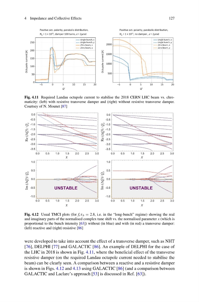
Fig. 4.11 Required Landau octupole current to stabilise the 2018 CERN LHC beam vs. chromaticity: (left) with resistive transverse damper and (right) without resistive transverse damper.
Courtsey of N. Mounet [87]
0.0
0.5
1.0
1.5
2.0
2.5
3.0
-3.5
-3.0
-2.5
-2.0
-1.5
-1.0
-0.5
0.0
0.0
0.5
1.0
1.5
2.0
2.5
3.0
-1.0
-0.5
0.0
0.5
1.0
0.0
0.5
1.0
1.5
2.0
2.5
3.0
-3.5
-3.0
-2.5
-2.0
-1.5
-1.0
-0.5
0.0
0.0
0.5
1.0
1.5
2.0
2.5
3.0
-1.0
-0.5
0.0
0.5
1.0
UNSTABLE
UNSTABLE
x
x
x
x
Im (∆Q /
Q
s
Re (∆Q
/
Q
s
)
Re (∆Q
/
Q
s
)
)
Im (∆Q /
Q
s
)
Fig. 4.12 Usual TMCI plots (for f r τ b = 2.8, i.e. in the “long-bunch” regime) showing the real
and imaginary parts of the normalised complex tune shift vs. the normalised parameter x (which is
proportional to the bunch intensity [63]) without (in blue) and with (in red) a transverse damper:
(left) reactive and (right) resistive [86]
were developed to take into account the effect of a transverse damper, such as NHT
[76], DELPHI [77] and GALACTIC [86]. An example of DELPHI for the case of
the LHC in 2018 is shown in Fig. 4.11, where the beneficial effect of the transverse
resistive damper (on the required Landau octupole current needed to stabilise the
beam) can be clearly seen. A comparison between a reactive and a resistive damper
is shown in Figs. 4.12 and 4.13 using GALACTIC [86] (and a comparison between
GALACTIC and Laclare’s approach [53] is discussed in Ref. [63]).
127
250
PosiƟve oct. polarity, parabolic distribuƟon,
N b = 1 × 10 11 , damper 100 turns, e = 2mrad
PosiƟve oct. polarity, parabolic distribuƟon,
N b = 1 × 10 11 , no damper , e = 2mrad
2000
single bunch, x
single bunch, y
25ns beam, x
25ns beam, y
single bunch, x
single bunch, y
25ns beam, x
25ns beam, y
1500
1000
500
200
150
100
Octupole current [A]
Octupole current [A]
50
0
–5
0
5
10
15
20
Q’
–5
0
5
10
15
20
Q’
Fig. 4.11 Required Landau octupole current to stabilise the 2018 CERN LHC beam vs. chromaticity: (left) with resistive transverse damper and (right) without resistive transverse damper.
Courtsey of N. Mounet [87]
0.0
0.5
1.0
1.5
2.0
2.5
3.0
-3.5
-3.0
-2.5
-2.0
-1.5
-1.0
-0.5
0.0
0.0
0.5
1.0
1.5
2.0
2.5
3.0
-1.0
-0.5
0.0
0.5
1.0
0.0
0.5
1.0
1.5
2.0
2.5
3.0
-3.5
-3.0
-2.5
-2.0
-1.5
-1.0
-0.5
0.0
0.0
0.5
1.0
1.5
2.0
2.5
3.0
-1.0
-0.5
0.0
0.5
1.0
UNSTABLE
UNSTABLE
x
x
x
x
Im (∆Q /
Q
s
Re (∆Q
/
Q
s
)
Re (∆Q
/
Q
s
)
)
Im (∆Q /
Q
s
)
Fig. 4.12 Usual TMCI plots (for f r τ b = 2.8, i.e. in the “long-bunch” regime) showing the real
and imaginary parts of the normalised complex tune shift vs. the normalised parameter x (which is
proportional to the bunch intensity [63]) without (in blue) and with (in red) a transverse damper:
(left) reactive and (right) resistive [86]
were developed to take into account the effect of a transverse damper, such as NHT
[76], DELPHI [77] and GALACTIC [86]. An example of DELPHI for the case of
the LHC in 2018 is shown in Fig. 4.11, where the beneficial effect of the transverse
resistive damper (on the required Landau octupole current needed to stabilise the
beam) can be clearly seen. A comparison between a reactive and a resistive damper
is shown in Figs. 4.12 and 4.13 using GALACTIC [86] (and a comparison between
GALACTIC and Laclare’s approach [53] is discussed in Ref. [63]).