

path for vehicle k should be chosen from the arc set A and only one arc can be
chosen. Constraints (3.3) guarantee that a path for vehicle k should be connected.
Specifically speaking, if x ka
t
¼ 1, that is, vehicle k chooses arc a as the tth link in a
path, then the next link in the path should have the starting node same as the ending
node of arc a. In other word, if x ka
t
¼ 0, then x ka
t+1
0 should be 0 for all arcs a
0 with
σ(a), δ(a
0 ). Constraints (3.4) force that a path of a vehicle k to start from the initial
node of the vehicle, i.e., l k . Constraints (3.5) count the transportation demand
fulfilled by a vehicle k. Constraints (3.6) ensure that the total transportation demand
for an arc a is split by all vehicles. Finally, constraints (3.7) define the domains for all
the decision variables.
However, it should be highlighted that the mathematical model listed above
cannot be directly used due to some technical limitations of the selected integer
programming modeling framework (i.e., for a vehicle k, x ka
t for all t T should be
well defined, but T is just an upper bound; therefore, if T is not appropriately chosen,
x ka
t for all t T cannot be well defined). To bypass such a modeling difficulty, a
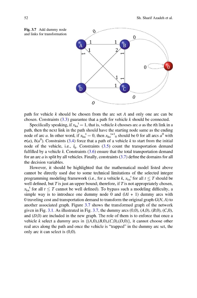
simple way is to introduce one dummy node 0 and (|A| + 1) dummy arcs with
0 traveling cost and transportation demand to transform the original graph G(N, A) to
another associated graph. Figure 3.7 shows the transformed graph of the network
given in Fig. 3.1. As illustrated in Fig. 3.7, the dummy arcs (0,0), (A,0), (B,0), (C,0),
and (D,0) are included in the new graph. The role of them is to enforce that once a
vehicle k select a dummy arcs in {(A,0),(B,0),(C,0),(D,0)}, it cannot choose other
real arcs along the path and once the vehicle is “trapped” in the dummy arc set, the
only arc it can select is (0,0).
Fig. 3.7 Add dummy node
and links for transformation
52
Sh. Sharif Azadeh et al.
chosen. Constraints (3.3) guarantee that a path for vehicle k should be connected.
Specifically speaking, if x ka
t
¼ 1, that is, vehicle k chooses arc a as the tth link in a
path, then the next link in the path should have the starting node same as the ending
node of arc a. In other word, if x ka
t
¼ 0, then x ka
t+1
0 should be 0 for all arcs a
0 with
σ(a), δ(a
0 ). Constraints (3.4) force that a path of a vehicle k to start from the initial
node of the vehicle, i.e., l k . Constraints (3.5) count the transportation demand
fulfilled by a vehicle k. Constraints (3.6) ensure that the total transportation demand
for an arc a is split by all vehicles. Finally, constraints (3.7) define the domains for all
the decision variables.
However, it should be highlighted that the mathematical model listed above
cannot be directly used due to some technical limitations of the selected integer
programming modeling framework (i.e., for a vehicle k, x ka
t for all t T should be
well defined, but T is just an upper bound; therefore, if T is not appropriately chosen,
x ka
t for all t T cannot be well defined). To bypass such a modeling difficulty, a
simple way is to introduce one dummy node 0 and (|A| + 1) dummy arcs with
0 traveling cost and transportation demand to transform the original graph G(N, A) to
another associated graph. Figure 3.7 shows the transformed graph of the network
given in Fig. 3.1. As illustrated in Fig. 3.7, the dummy arcs (0,0), (A,0), (B,0), (C,0),
and (D,0) are included in the new graph. The role of them is to enforce that once a
vehicle k select a dummy arcs in {(A,0),(B,0),(C,0),(D,0)}, it cannot choose other
real arcs along the path and once the vehicle is “trapped” in the dummy arc set, the
only arc it can select is (0,0).
Fig. 3.7 Add dummy node
and links for transformation
52
Sh. Sharif Azadeh et al.