

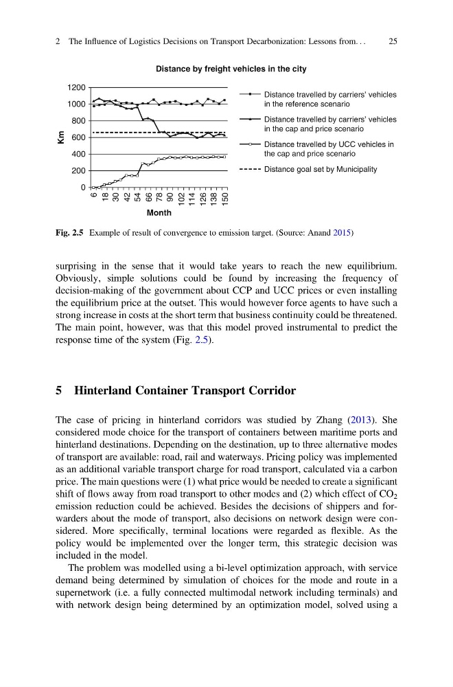
surprising in the sense that it would take years to reach the new equilibrium.
Obviously, simple solutions could be found by increasing the frequency of
decision-making of the government about CCP and UCC prices or even installing
the equilibrium price at the outset. This would however force agents to have such a
strong increase in costs at the short term that business continuity could be threatened.
The main point, however, was that this model proved instrumental to predict the
response time of the system (Fig. 2.5).
5 Hinterland Container Transport Corridor
The case of pricing in hinterland corridors was studied by Zhang (2013). She
considered mode choice for the transport of containers between maritime ports and
hinterland destinations. Depending on the destination, up to three alternative modes
of transport are available: road, rail and waterways. Pricing policy was implemented
as an additional variable transport charge for road transport, calculated via a carbon
price. The main questions were (1) what price would be needed to create a significant
shift of flows away from road transport to other modes and (2) which effect of CO 2
emission reduction could be achieved. Besides the decisions of shippers and forwarders about the mode of transport, also decisions on network design were considered. More specifically, terminal locations were regarded as flexible. As the
policy would be implemented over the longer term, this strategic decision was
included in the model.
The problem was modelled using a bi-level optimization approach, with service
demand being determined by simulation of choices for the mode and route in a
supernetwork (i.e. a fully connected multimodal network including terminals) and
with network design being determined by an optimization model, solved using a
1200
Distance by freight vehicles in the city
Distance travelled by carriers’ vehicles
in the reference scenario
Distance travelled by carriers’ vehicles
in the cap and price scenario
Distance travelled by UCC vehicles in
the cap and price scenario
Distance goal set by Municipality
1000
800
600
400
200
Month
Km
0
6
18
30
42
54
66
78
90
102
114
126
138
150
Fig. 2.5 Example of result of convergence to emission target. (Source: Anand 2015)
2 The Influence of Logistics Decisions on Transport Decarbonization: Lessons from. . .
25
Obviously, simple solutions could be found by increasing the frequency of
decision-making of the government about CCP and UCC prices or even installing
the equilibrium price at the outset. This would however force agents to have such a
strong increase in costs at the short term that business continuity could be threatened.
The main point, however, was that this model proved instrumental to predict the
response time of the system (Fig. 2.5).
5 Hinterland Container Transport Corridor
The case of pricing in hinterland corridors was studied by Zhang (2013). She
considered mode choice for the transport of containers between maritime ports and
hinterland destinations. Depending on the destination, up to three alternative modes
of transport are available: road, rail and waterways. Pricing policy was implemented
as an additional variable transport charge for road transport, calculated via a carbon
price. The main questions were (1) what price would be needed to create a significant
shift of flows away from road transport to other modes and (2) which effect of CO 2
emission reduction could be achieved. Besides the decisions of shippers and forwarders about the mode of transport, also decisions on network design were considered. More specifically, terminal locations were regarded as flexible. As the
policy would be implemented over the longer term, this strategic decision was
included in the model.
The problem was modelled using a bi-level optimization approach, with service
demand being determined by simulation of choices for the mode and route in a
supernetwork (i.e. a fully connected multimodal network including terminals) and
with network design being determined by an optimization model, solved using a
1200
Distance by freight vehicles in the city
Distance travelled by carriers’ vehicles
in the reference scenario
Distance travelled by carriers’ vehicles
in the cap and price scenario
Distance travelled by UCC vehicles in
the cap and price scenario
Distance goal set by Municipality
1000
800
600
400
200
Month
Km
0
6
18
30
42
54
66
78
90
102
114
126
138
150
Fig. 2.5 Example of result of convergence to emission target. (Source: Anand 2015)
2 The Influence of Logistics Decisions on Transport Decarbonization: Lessons from. . .
25