

13 If Truncated Wave Functions of Excited State Energy Saddle Points Are. . .
505
“false”-converged δp in order to send it farther to n = 2, i.e., “before” the crossing
where the real minimum should be [cf. Table 13.8]. (Such a “false” convergence
should always be checked). While being in n = 1, it approached p = (2.34, 0.94,
1.01); in order to send it farther to n = 2 “before” the crossing, p was extrapolated
every three steps by twice the final step – or more if convergence is slow, according
to the logical code exposed in Table 13.2. Such an extrapolation was also used in
the first example above; in the second it was not needed.
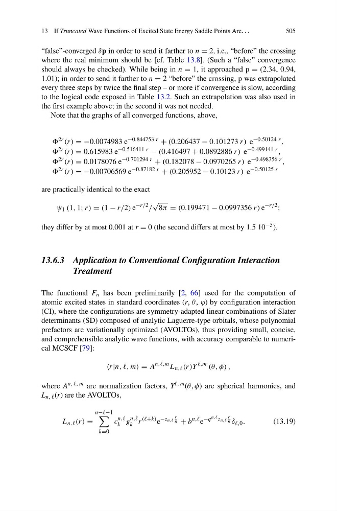
Note that the graphs of all converged functions, above,
2r (r) = −0.0074983 e −0.844753 r + (0.206437 − 0.101273 r) e −0.50124 r ,
2r (r) = 0.615983 e −0.516411 r − (0.416497 + 0.0892886 r) e −0.499141 r ,
2r (r) = 0.0178076 e −0.701294 r + (0.182078 − 0.0970265 r) e −0.498356 r ,
2r (r) = −0.00706569 e −0.87182 r + (0.205952 − 0.10123 r) e −0.50125 r
are practically identical to the exact
ψ 1 (1, 1; r) = (1 − r/2) e
−r/2 /
√
8π = (0.199471 − 0.0997356 r) e
−r/2
;
they differ by at most 0.001 at r = 0 (the second differs at most by 1.5 10 −5 ).
13.6.3 Application to Conventional Configuration Interaction
Treatment
The functional F n has been preliminarily [2, 66] used for the computation of
atomic excited states in standard coordinates (r, θ , ϕ) by configuration interaction
(CI), where the configurations are symmetry-adapted linear combinations of Slater
determinants (SD) composed of analytic Laguerre-type orbitals, whose polynomial
prefactors are variationally optimized (AVOLTOs), thus providing small, concise,
and comprehensible analytic wave functions, with accuracy comparable to numerical MCSCF [79]:
r|n, ,, m = A
n,,,m L n,, (r)Y
,m (θ, φ) ,
where A n, , m are normalization factors, Y , m (θ , φ) are spherical harmonics, and
L n, (r) are the AVOLTOs,
L n,, (r) =
n−−1
k=0
c
n,,
k g
n,,
k r
(+k) e
−z n,,
r
n + b
n,, e
−q n,, z n,,
r
n δ ,0 .
(13.19)
505
“false”-converged δp in order to send it farther to n = 2, i.e., “before” the crossing
where the real minimum should be [cf. Table 13.8]. (Such a “false” convergence
should always be checked). While being in n = 1, it approached p = (2.34, 0.94,
1.01); in order to send it farther to n = 2 “before” the crossing, p was extrapolated
every three steps by twice the final step – or more if convergence is slow, according
to the logical code exposed in Table 13.2. Such an extrapolation was also used in
the first example above; in the second it was not needed.
Note that the graphs of all converged functions, above,
2r (r) = −0.0074983 e −0.844753 r + (0.206437 − 0.101273 r) e −0.50124 r ,
2r (r) = 0.615983 e −0.516411 r − (0.416497 + 0.0892886 r) e −0.499141 r ,
2r (r) = 0.0178076 e −0.701294 r + (0.182078 − 0.0970265 r) e −0.498356 r ,
2r (r) = −0.00706569 e −0.87182 r + (0.205952 − 0.10123 r) e −0.50125 r
are practically identical to the exact
ψ 1 (1, 1; r) = (1 − r/2) e
−r/2 /
√
8π = (0.199471 − 0.0997356 r) e
−r/2
;
they differ by at most 0.001 at r = 0 (the second differs at most by 1.5 10 −5 ).
13.6.3 Application to Conventional Configuration Interaction
Treatment
The functional F n has been preliminarily [2, 66] used for the computation of
atomic excited states in standard coordinates (r, θ , ϕ) by configuration interaction
(CI), where the configurations are symmetry-adapted linear combinations of Slater
determinants (SD) composed of analytic Laguerre-type orbitals, whose polynomial
prefactors are variationally optimized (AVOLTOs), thus providing small, concise,
and comprehensible analytic wave functions, with accuracy comparable to numerical MCSCF [79]:
r|n, ,, m = A
n,,,m L n,, (r)Y
,m (θ, φ) ,
where A n, , m are normalization factors, Y , m (θ , φ) are spherical harmonics, and
L n, (r) are the AVOLTOs,
L n,, (r) =
n−−1
k=0
c
n,,
k g
n,,
k r
(+k) e
−z n,,
r
n + b
n,, e
−q n,, z n,,
r
n δ ,0 .
(13.19)