

180
S. Taioli
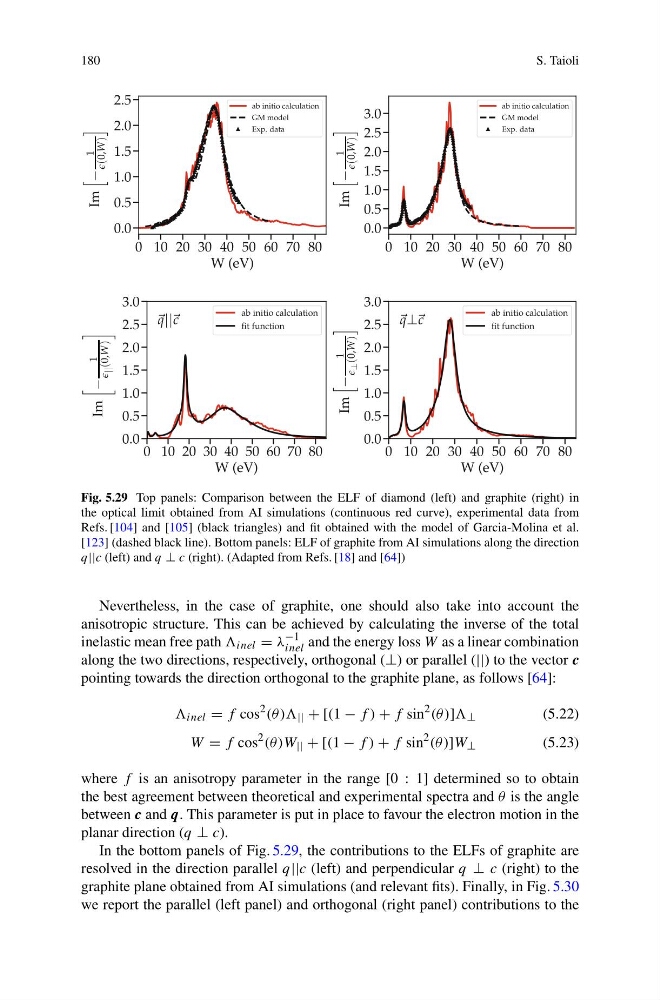
Fig. 5.29 Top panels: Comparison between the ELF of diamond (left) and graphite (right) in
the optical limit obtained from AI simulations (continuous red curve), experimental data from
Refs. [104] and [105] (black triangles) and fit obtained with the model of Garcia-Molina et al.
[123] (dashed black line). Bottom panels: ELF of graphite from AI simulations along the direction
q||c (left) and q ⊥ c (right). (Adapted from Refs. [18] and [64])
Nevertheless, in the case of graphite, one should also take into account the
anisotropic structure. This can be achieved by calculating the inverse of the total
inelastic mean free path inel = λ
−1
inel and the energy loss W as a linear combination
along the two directions, respectively, orthogonal (⊥) or parallel (||) to the vector c
pointing towards the direction orthogonal to the graphite plane, as follows [64]:
inel = f cos
2 (θ )) || + [(1 − f ) + f sin
2 (θ )] ⊥
(5.22)
W = f cos
2 (θ )W || + [(1 − f ) + f sin
2 (θ )]W ⊥
(5.23)
where f is an anisotropy parameter in the range [0 : 1] determined so to obtain
the best agreement between theoretical and experimental spectra and θ is the angle
between c and q. This parameter is put in place to favour the electron motion in the
planar direction (q ⊥ c).
In the bottom panels of Fig. 5.29, the contributions to the ELFs of graphite are
resolved in the direction parallel q||c (left) and perpendicular q ⊥ c (right) to the
graphite plane obtained from AI simulations (and relevant fits). Finally, in Fig. 5.30
we report the parallel (left panel) and orthogonal (right panel) contributions to the
S. Taioli
Fig. 5.29 Top panels: Comparison between the ELF of diamond (left) and graphite (right) in
the optical limit obtained from AI simulations (continuous red curve), experimental data from
Refs. [104] and [105] (black triangles) and fit obtained with the model of Garcia-Molina et al.
[123] (dashed black line). Bottom panels: ELF of graphite from AI simulations along the direction
q||c (left) and q ⊥ c (right). (Adapted from Refs. [18] and [64])
Nevertheless, in the case of graphite, one should also take into account the
anisotropic structure. This can be achieved by calculating the inverse of the total
inelastic mean free path inel = λ
−1
inel and the energy loss W as a linear combination
along the two directions, respectively, orthogonal (⊥) or parallel (||) to the vector c
pointing towards the direction orthogonal to the graphite plane, as follows [64]:
inel = f cos
2 (θ )) || + [(1 − f ) + f sin
2 (θ )] ⊥
(5.22)
W = f cos
2 (θ )W || + [(1 − f ) + f sin
2 (θ )]W ⊥
(5.23)
where f is an anisotropy parameter in the range [0 : 1] determined so to obtain
the best agreement between theoretical and experimental spectra and θ is the angle
between c and q. This parameter is put in place to favour the electron motion in the
planar direction (q ⊥ c).
In the bottom panels of Fig. 5.29, the contributions to the ELFs of graphite are
resolved in the direction parallel q||c (left) and perpendicular q ⊥ c (right) to the
graphite plane obtained from AI simulations (and relevant fits). Finally, in Fig. 5.30
we report the parallel (left panel) and orthogonal (right panel) contributions to the