

382
In this chapter, I have calculated the “global carbon budget” and the “global CO 2
concentration,” and, by determining the amount of CO 2 being input to the atmosphere relative to the global CO 2 balance, the rate of acceleration of atmospheric
CO 2 emissions annually. Furthermore, I have prepared detailed data sets using
MATLAB software and have calculated the annual total global carbon emissions
from the preindustrial period (1750) to the modern period (2015). All CO 2 emissions from the burning of fossil fuel and land-use change from 1750 to the industrial
revolution and from 1870 to the modern era have been analyzed in detail by incorporating data from the Fifth Assessment Report of the Intergovernmental Panel on
Climate Change (IPCC AR5) into MATLAB software to ensure the most accurate
estimates of CO 2 emissions into the atmosphere since this gas is the major driver of
climate change. The estimated CO 2 emissions from burning fossil fuel are referred
to as E FF ; Gt/year, and the emissions resulting from land-use change are E LUC ; Gt/
year. The sequestration and the absorption of CO 2 by the oceans, which is referred
to as S OCEAN ; Gt/year, and by the terrestrial vegetation, which is referred to as S LAND ;
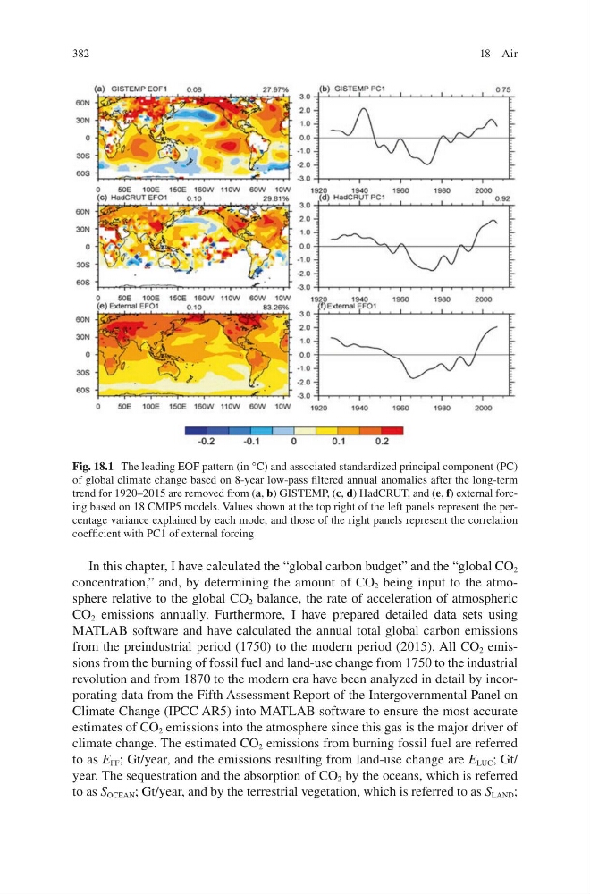
Fig. 18.1 The leading EOF pattern (in °C) and associated standardized principal component (PC)
of global climate change based on 8-year low-pass filtered annual anomalies after the long-term
trend for 1920–2015 are removed from (a, b) GISTEMP, (c, d) HadCRUT, and (e, f) external forcing based on 18 CMIP5 models. Values shown at the top right of the left panels represent the percentage variance explained by each mode, and those of the right panels represent the correlation
coefficient with PC1 of external forcing
18 Air
In this chapter, I have calculated the “global carbon budget” and the “global CO 2
concentration,” and, by determining the amount of CO 2 being input to the atmosphere relative to the global CO 2 balance, the rate of acceleration of atmospheric
CO 2 emissions annually. Furthermore, I have prepared detailed data sets using
MATLAB software and have calculated the annual total global carbon emissions
from the preindustrial period (1750) to the modern period (2015). All CO 2 emissions from the burning of fossil fuel and land-use change from 1750 to the industrial
revolution and from 1870 to the modern era have been analyzed in detail by incorporating data from the Fifth Assessment Report of the Intergovernmental Panel on
Climate Change (IPCC AR5) into MATLAB software to ensure the most accurate
estimates of CO 2 emissions into the atmosphere since this gas is the major driver of
climate change. The estimated CO 2 emissions from burning fossil fuel are referred
to as E FF ; Gt/year, and the emissions resulting from land-use change are E LUC ; Gt/
year. The sequestration and the absorption of CO 2 by the oceans, which is referred
to as S OCEAN ; Gt/year, and by the terrestrial vegetation, which is referred to as S LAND ;
Fig. 18.1 The leading EOF pattern (in °C) and associated standardized principal component (PC)
of global climate change based on 8-year low-pass filtered annual anomalies after the long-term
trend for 1920–2015 are removed from (a, b) GISTEMP, (c, d) HadCRUT, and (e, f) external forcing based on 18 CMIP5 models. Values shown at the top right of the left panels represent the percentage variance explained by each mode, and those of the right panels represent the correlation
coefficient with PC1 of external forcing
18 Air