

372
the sky. Thus, the model is developed by kinetic force producing energy for the flying train control mechanism by governing the mechanical power control as below:
P
C
AV
w
p
,
=
( )
1
2
3
λ β ρ
(17.23)
where ρ is the air density (kg/m
3
), C p is the power coefficient, A is the intercepting
area of the flying train (m
2
), V is the average speed (m/s), and λ is the tip speed ratio
[31]. The theoretical maximum value of the power coefficient C p is 0.593; C p is also
known as Betz’s coefficient. Mathematically,
λ
ω
=
R
V
(17.24)
R is the radius of the flying train (m), ω is the speed (rad/s), and V is the average
speed (m/s) and thus the net energy required by the flying train is calculated as
Q
P
w
Time kWh
= ×(
)[
]
(17.25)
Since wind velocity has some impact on flying train, a direct measurement of
wind speed has also been calculated considering any particular motion when the
train will be flying and thus the motion of the flying train has been determined considering its maximum flying height to run the flying train in the sky smoothly:
v Z
Z
Z
v Z
Z
Z
( )
= ( )
ln
ln
r
r
0
0
(17.26)
where Z r is the flying height (m), Z is the height to be determined, Z 0 is the measure of
surface roughness (0.1–0.25 for crop land), v(Z) is the flying train speed at height z
(m/s), and v(Z r ) is the wind speed at the reference height z (m/s) (Fig. 17.4). The
power output in terms of the flying train shall be estimated using the following
equation:
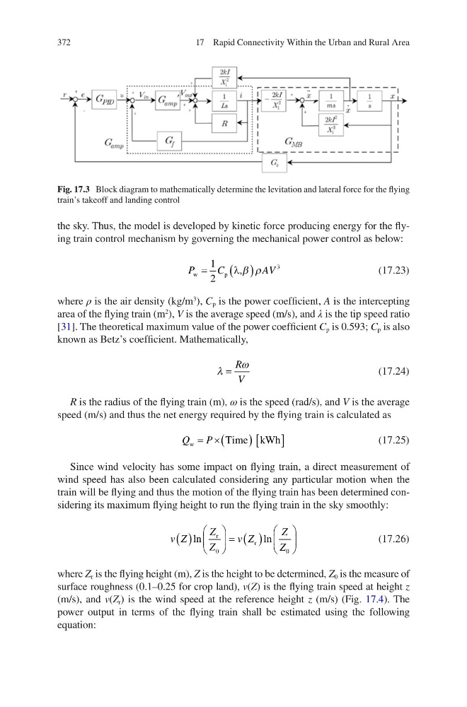
Fig. 17.3 Block diagram to mathematically determine the levitation and lateral force for the flying
train’s takeoff and landing control
17 Rapid Connectivity Within the Urban and Rural Area
the sky. Thus, the model is developed by kinetic force producing energy for the flying train control mechanism by governing the mechanical power control as below:
P
C
AV
w
p
,
=
( )
1
2
3
λ β ρ
(17.23)
where ρ is the air density (kg/m
3
), C p is the power coefficient, A is the intercepting
area of the flying train (m
2
), V is the average speed (m/s), and λ is the tip speed ratio
[31]. The theoretical maximum value of the power coefficient C p is 0.593; C p is also
known as Betz’s coefficient. Mathematically,
λ
ω
=
R
V
(17.24)
R is the radius of the flying train (m), ω is the speed (rad/s), and V is the average
speed (m/s) and thus the net energy required by the flying train is calculated as
Q
P
w
Time kWh
= ×(
)[
]
(17.25)
Since wind velocity has some impact on flying train, a direct measurement of
wind speed has also been calculated considering any particular motion when the
train will be flying and thus the motion of the flying train has been determined considering its maximum flying height to run the flying train in the sky smoothly:
v Z
Z
Z
v Z
Z
Z
( )
= ( )
ln
ln
r
r
0
0
(17.26)
where Z r is the flying height (m), Z is the height to be determined, Z 0 is the measure of
surface roughness (0.1–0.25 for crop land), v(Z) is the flying train speed at height z
(m/s), and v(Z r ) is the wind speed at the reference height z (m/s) (Fig. 17.4). The
power output in terms of the flying train shall be estimated using the following
equation:
Fig. 17.3 Block diagram to mathematically determine the levitation and lateral force for the flying
train’s takeoff and landing control
17 Rapid Connectivity Within the Urban and Rural Area