

369
number contours for a safe physical model of a flying train by implementing a 3D
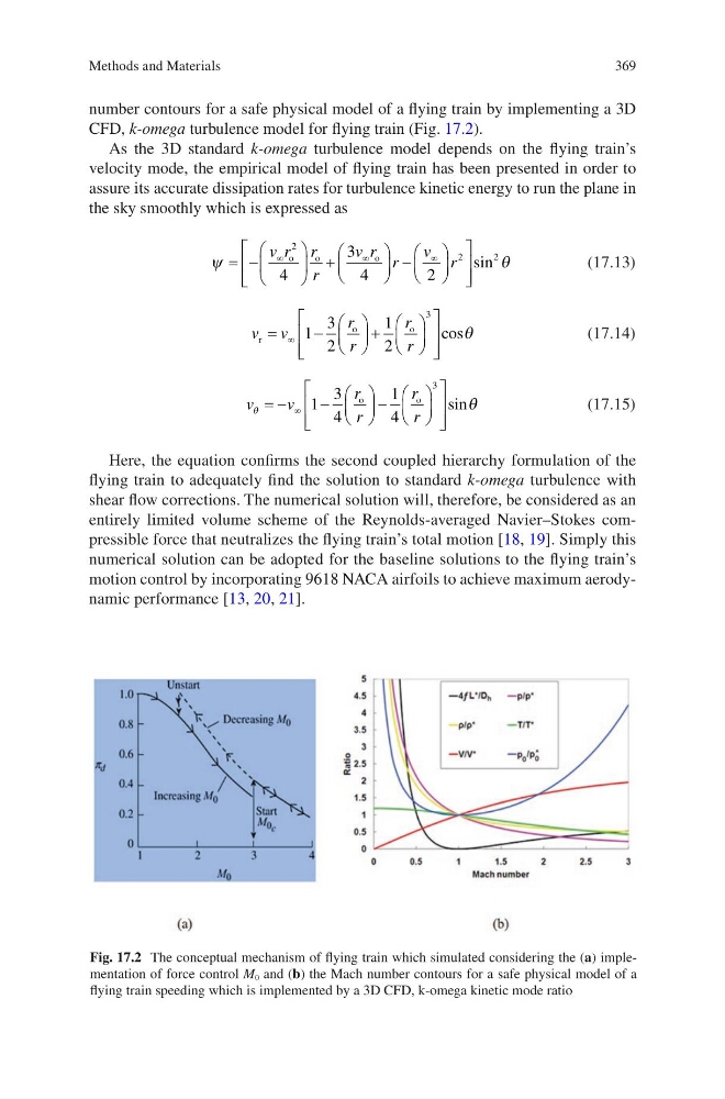
CFD, k-omega turbulence model for flying train (Fig. 17.2).
As the 3D standard k-omega turbulence model depends on the flying train’s
velocity mode, the empirical model of flying train has been presented in order to
assure its accurate dissipation rates for turbulence kinetic energy to run the plane in
the sky smoothly which is expressed as
ψ
θ
= −
+
−
∞
∞
∞
v r r
r
v r r
v r
o
o
o
2
2
2
4
3
4
2
sin
(17.13)
v v
r
r
r
r
r
o
o
=
−
+
∞ 1
3
2
1
2
3
cosθ
(17.14)
v
v
r
r
r
r
θ
θ
= −
−
−
∞ 1
3
4
1
4
3
o
o
sin
(17.15)
Here, the equation confirms the second coupled hierarchy formulation of the
flying train to adequately find the solution to standard k-omega turbulence with
shear flow corrections. The numerical solution will, therefore, be considered as an
entirely limited volume scheme of the Reynolds-averaged Navier–Stokes compressible force that neutralizes the flying train’s total motion [18, 19]. Simply this
numerical solution can be adopted for the baseline solutions to the flying train’s
motion control by incorporating 9618 NACA airfoils to achieve maximum aerodynamic performance [13, 20, 21].
Fig. 17.2 The conceptual mechanism of flying train which simulated considering the (a) implementation of force control M 0 and (b) the Mach number contours for a safe physical model of a
flying train speeding which is implemented by a 3D CFD, k-omega kinetic mode ratio
Methods and Materials
number contours for a safe physical model of a flying train by implementing a 3D
CFD, k-omega turbulence model for flying train (Fig. 17.2).
As the 3D standard k-omega turbulence model depends on the flying train’s
velocity mode, the empirical model of flying train has been presented in order to
assure its accurate dissipation rates for turbulence kinetic energy to run the plane in
the sky smoothly which is expressed as
ψ
θ
= −
+
−
∞
∞
∞
v r r
r
v r r
v r
o
o
o
2
2
2
4
3
4
2
sin
(17.13)
v v
r
r
r
r
r
o
o
=
−
+
∞ 1
3
2
1
2
3
cosθ
(17.14)
v
v
r
r
r
r
θ
θ
= −
−
−
∞ 1
3
4
1
4
3
o
o
sin
(17.15)
Here, the equation confirms the second coupled hierarchy formulation of the
flying train to adequately find the solution to standard k-omega turbulence with
shear flow corrections. The numerical solution will, therefore, be considered as an
entirely limited volume scheme of the Reynolds-averaged Navier–Stokes compressible force that neutralizes the flying train’s total motion [18, 19]. Simply this
numerical solution can be adopted for the baseline solutions to the flying train’s
motion control by incorporating 9618 NACA airfoils to achieve maximum aerodynamic performance [13, 20, 21].
Fig. 17.2 The conceptual mechanism of flying train which simulated considering the (a) implementation of force control M 0 and (b) the Mach number contours for a safe physical model of a
flying train speeding which is implemented by a 3D CFD, k-omega kinetic mode ratio
Methods and Materials