

60
P. Liu
Using the above formula and absorbing the proportional coefficient into
the mixing length l m , we can get the result.
τ t = −ρu ν = ρl
2
m
∂u
∂ y
∂u
∂ y
, ν t = l
2
m
∂u
∂ y
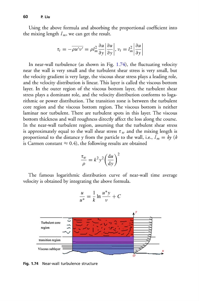
In near-wall turbulence (as shown in Fig. 1.74), the fluctuating velocity
near the wall is very small and the turbulent shear stress is very small, but
the velocity gradient is very large, the viscous shear stress plays a leading role,
and the velocity distribution is linear. This layer is called the viscous bottom
layer. In the outer region of the viscous bottom layer, the turbulent shear
stress plays a dominant role, and the velocity distribution conforms to logarithmic or power distribution. The transition zone is between the turbulent
core region and the viscous bottom region. The viscous bottom is neither
laminar nor turbulent. There are turbulent spots in this layer. The viscous
bottom thickness and wall roughness directly affect the loss along the course.
In the near-wall turbulent region, assuming that the turbulent shear stress
is approximately equal to the wall shear stress τ w and the mixing length is
proportional to the distance y from the particle to the wall, i.e., l m = ky (k
is Carmen constant ≈ 0.4), the following results are obtained
τ w
ρ
= k
2 y
2
du
dy
2
The famous logarithmic distribution curve of near-wall time average
velocity is obtained by integrating the above formula.
u
u ∗ =
1
k
ln
u ∗ y
ν
+ C
Fig. 1.74 Near-wall turbulence structure
P. Liu
Using the above formula and absorbing the proportional coefficient into
the mixing length l m , we can get the result.
τ t = −ρu ν = ρl
2
m
∂u
∂ y
∂u
∂ y
, ν t = l
2
m
∂u
∂ y
In near-wall turbulence (as shown in Fig. 1.74), the fluctuating velocity
near the wall is very small and the turbulent shear stress is very small, but
the velocity gradient is very large, the viscous shear stress plays a leading role,
and the velocity distribution is linear. This layer is called the viscous bottom
layer. In the outer region of the viscous bottom layer, the turbulent shear
stress plays a dominant role, and the velocity distribution conforms to logarithmic or power distribution. The transition zone is between the turbulent
core region and the viscous bottom region. The viscous bottom is neither
laminar nor turbulent. There are turbulent spots in this layer. The viscous
bottom thickness and wall roughness directly affect the loss along the course.
In the near-wall turbulent region, assuming that the turbulent shear stress
is approximately equal to the wall shear stress τ w and the mixing length is
proportional to the distance y from the particle to the wall, i.e., l m = ky (k
is Carmen constant ≈ 0.4), the following results are obtained
τ w
ρ
= k
2 y
2
du
dy
2
The famous logarithmic distribution curve of near-wall time average
velocity is obtained by integrating the above formula.
u
u ∗ =
1
k
ln
u ∗ y
ν
+ C
Fig. 1.74 Near-wall turbulence structure