

r
2 x
0
ðjÞ ¼
1
n
X j¼1
n
x
0
ðjÞ À x 0 ðjÞ
2 ¼
1
n
X j¼1
n
x
0
ðjÞ
ð
Þ
2 ¼ x 02 ðjÞ ¼ ACFð0Þ
ð3:144Þ
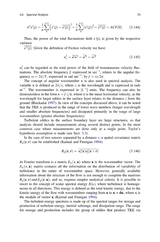
Thus, the power of the total fluctuations field x’(j), is given by the respective
variance
x
0 2 ðjÞ. Given the definition of friction velocity we have:
u
2
à ¼ u 0 w 0 ¼ u 02 ¼ w 02
ð3:145Þ
u
2
à can be regarded as the total power of the field of instantaneous velocity fluctuations. The absolute frequency f, expressed in sec
−1 , relates to the angular frequency x ¼ 2p=T, expressed in rad sec
−1 , by f ¼ x=2p.
The concept of angular wavenumber j is also used in spectral analysis. The
variable j is defined as 2p=k, where k is the wavelength and is expressed in rads
m
−1 . The wavenumber is expressed in L
À1
½ units. The frequency can also be
dimensionless in the form n ¼ f z=u, where u is the mean horizontal velocity, as the
wavelength for larger eddies in the surface layer relates to the distance z from the
ground (Blackadar 1997). In view of the concepts discussed above, it can be noted
that the TKE is produced in the range of lower wave numbers (longer wavelength
and smaller absolute frequencies) and dissipated primarily in the range of large
wavenumbers (greater absolute frequencies).
Turbulent eddies in the surface boundary layer are large structures, so that
analysis should include measurements along several distinct points. In the most
common case where measurements are done only at a single point, Taylor’s
hypothesis assumption is made (see Sect. 3.3).
In the case of two sensors separated by a distance r, a spatial covariance matrix
R ij ðx; rÞ can be established (Kaimal and Finnigan 1994):
R ij ðx; rÞ ¼ u 0
i ðxÞu 0
j ðx þ rÞ
ð 3:146Þ
its Fourier transform is a matrix E ij ðx; jÞ where j is the wavenumber vector. The
E ij ðx; jÞ matrix contains all the information on the distribution of variability of
turbulence in the entire of wavenumber space. However, generally available
information about the structure of the flow is not enough to complete the matrixes
R ij ðx; rÞ and E ij ðx; jÞ, and so, requires simpler analytical criteria. It is possible to
resort to the concept of scalar spectral energy E(j), where turbulence is homogeneous in all directions. This energy is defined as the total kinetic energy, due to the
kinetic energy of the flow with wavenumbers ranging from j to j + dj, where j is
the module of vector j (Kaimal and Finnigan 1994).
The turbulent energy spectrum is made up of the spectral ranges for storage and
production of turbulent energy, inertial subrange, and dissipation range. The range
for storage and production includes the group of eddies that produce TKE via
3.6 Spectral Analysis
73
2 x
0
ðjÞ ¼
1
n
X j¼1
n
x
0
ðjÞ À x 0 ðjÞ
2 ¼
1
n
X j¼1
n
x
0
ðjÞ
ð
Þ
2 ¼ x 02 ðjÞ ¼ ACFð0Þ
ð3:144Þ
Thus, the power of the total fluctuations field x’(j), is given by the respective
variance
x
0 2 ðjÞ. Given the definition of friction velocity we have:
u
2
à ¼ u 0 w 0 ¼ u 02 ¼ w 02
ð3:145Þ
u
2
à can be regarded as the total power of the field of instantaneous velocity fluctuations. The absolute frequency f, expressed in sec
−1 , relates to the angular frequency x ¼ 2p=T, expressed in rad sec
−1 , by f ¼ x=2p.
The concept of angular wavenumber j is also used in spectral analysis. The
variable j is defined as 2p=k, where k is the wavelength and is expressed in rads
m
−1 . The wavenumber is expressed in L
À1
½ units. The frequency can also be
dimensionless in the form n ¼ f z=u, where u is the mean horizontal velocity, as the
wavelength for larger eddies in the surface layer relates to the distance z from the
ground (Blackadar 1997). In view of the concepts discussed above, it can be noted
that the TKE is produced in the range of lower wave numbers (longer wavelength
and smaller absolute frequencies) and dissipated primarily in the range of large
wavenumbers (greater absolute frequencies).
Turbulent eddies in the surface boundary layer are large structures, so that
analysis should include measurements along several distinct points. In the most
common case where measurements are done only at a single point, Taylor’s
hypothesis assumption is made (see Sect. 3.3).
In the case of two sensors separated by a distance r, a spatial covariance matrix
R ij ðx; rÞ can be established (Kaimal and Finnigan 1994):
R ij ðx; rÞ ¼ u 0
i ðxÞu 0
j ðx þ rÞ
ð 3:146Þ
its Fourier transform is a matrix E ij ðx; jÞ where j is the wavenumber vector. The
E ij ðx; jÞ matrix contains all the information on the distribution of variability of
turbulence in the entire of wavenumber space. However, generally available
information about the structure of the flow is not enough to complete the matrixes
R ij ðx; rÞ and E ij ðx; jÞ, and so, requires simpler analytical criteria. It is possible to
resort to the concept of scalar spectral energy E(j), where turbulence is homogeneous in all directions. This energy is defined as the total kinetic energy, due to the
kinetic energy of the flow with wavenumbers ranging from j to j + dj, where j is
the module of vector j (Kaimal and Finnigan 1994).
The turbulent energy spectrum is made up of the spectral ranges for storage and
production of turbulent energy, inertial subrange, and dissipation range. The range
for storage and production includes the group of eddies that produce TKE via
3.6 Spectral Analysis
73