

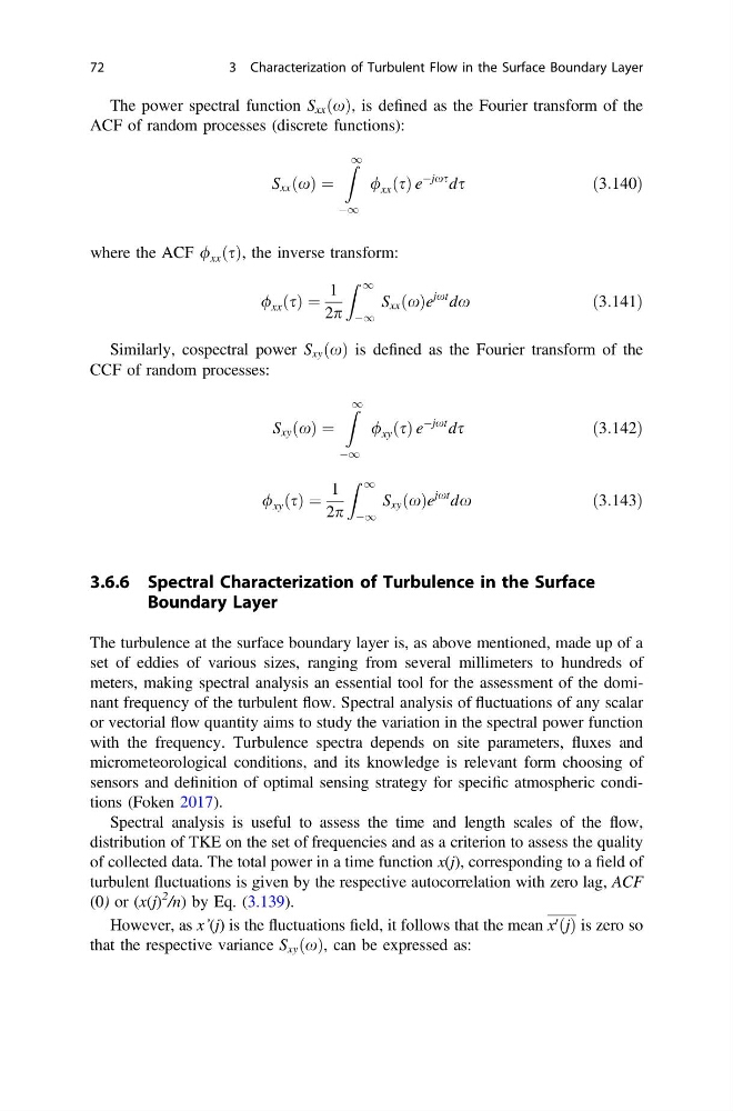
The power spectral function S xx ðxÞ, is defined as the Fourier transform of the
ACF of random processes (discrete functions):
S xx ðxÞ ¼
Z 1
À1
/ xx ðsÞ e
Àjxs ds
ð3:140Þ
where the ACF / xx ðsÞ, the inverse transform:
/ xx ðsÞ ¼
1
2p
Z 1
À1
S xx ðxÞe
jxt dx
ð3:141Þ
Similarly, cospectral power S xy ðxÞ is defined as the Fourier transform of the
CCF of random processes:
S xy ðxÞ ¼
Z 1
À1
/ xy ðsÞ e
Àjxt ds
ð3:142Þ
/ xy ðsÞ ¼
1
2p
Z 1
À1
S xy ðxÞe
jxt dx
ð3:143Þ
3.6.6 Spectral Characterization of Turbulence in the Surface
Boundary Layer
The turbulence at the surface boundary layer is, as above mentioned, made up of a
set of eddies of various sizes, ranging from several millimeters to hundreds of
meters, making spectral analysis an essential tool for the assessment of the dominant frequency of the turbulent flow. Spectral analysis of fluctuations of any scalar
or vectorial flow quantity aims to study the variation in the spectral power function
with the frequency. Turbulence spectra depends on site parameters, fluxes and
micrometeorological conditions, and its knowledge is relevant form choosing of
sensors and definition of optimal sensing strategy for specific atmospheric conditions (Foken 2017).
Spectral analysis is useful to assess the time and length scales of the flow,
distribution of TKE on the set of frequencies and as a criterion to assess the quality
of collected data. The total power in a time function x(j), corresponding to a field of
turbulent fluctuations is given by the respective autocorrelation with zero lag, ACF
(0) or (x(j)
2 /n) by Eq. (3.139).
However, as x’(j) is the fluctuations field, it follows that the mean x 0 ðjÞ is zero so
that the respective variance S xy ðxÞ, can be expressed as:
72
3 Characterization of Turbulent Flow in the Surface Boundary Layer
ACF of random processes (discrete functions):
S xx ðxÞ ¼
Z 1
À1
/ xx ðsÞ e
Àjxs ds
ð3:140Þ
where the ACF / xx ðsÞ, the inverse transform:
/ xx ðsÞ ¼
1
2p
Z 1
À1
S xx ðxÞe
jxt dx
ð3:141Þ
Similarly, cospectral power S xy ðxÞ is defined as the Fourier transform of the
CCF of random processes:
S xy ðxÞ ¼
Z 1
À1
/ xy ðsÞ e
Àjxt ds
ð3:142Þ
/ xy ðsÞ ¼
1
2p
Z 1
À1
S xy ðxÞe
jxt dx
ð3:143Þ
3.6.6 Spectral Characterization of Turbulence in the Surface
Boundary Layer
The turbulence at the surface boundary layer is, as above mentioned, made up of a
set of eddies of various sizes, ranging from several millimeters to hundreds of
meters, making spectral analysis an essential tool for the assessment of the dominant frequency of the turbulent flow. Spectral analysis of fluctuations of any scalar
or vectorial flow quantity aims to study the variation in the spectral power function
with the frequency. Turbulence spectra depends on site parameters, fluxes and
micrometeorological conditions, and its knowledge is relevant form choosing of
sensors and definition of optimal sensing strategy for specific atmospheric conditions (Foken 2017).
Spectral analysis is useful to assess the time and length scales of the flow,
distribution of TKE on the set of frequencies and as a criterion to assess the quality
of collected data. The total power in a time function x(j), corresponding to a field of
turbulent fluctuations is given by the respective autocorrelation with zero lag, ACF
(0) or (x(j)
2 /n) by Eq. (3.139).
However, as x’(j) is the fluctuations field, it follows that the mean x 0 ðjÞ is zero so
that the respective variance S xy ðxÞ, can be expressed as:
72
3 Characterization of Turbulent Flow in the Surface Boundary Layer