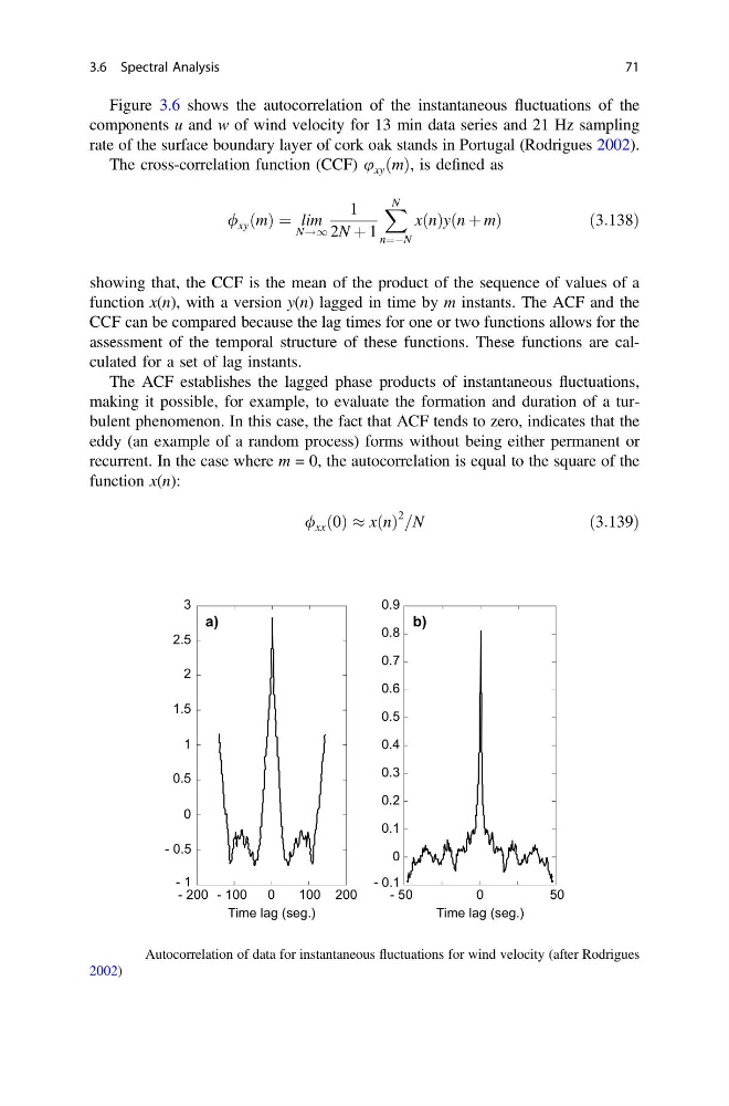
Figure 3.6 shows the autocorrelation of the instantaneous fluctuations of the
components u and w of wind velocity for 13 min data series and 21 Hz sampling
rate of the surface boundary layer of cork oak stands in Portugal (Rodrigues 2002).
The cross-correlation function (CCF) u xy ðmÞ, is defined as
/ xy ðmÞ ¼ lim
N!1
1
2N þ 1
X N
n¼ÀN
xðnÞyðn þ mÞ
ð 3:138Þ
showing that, the CCF is the mean of the product of the sequence of values of a
function x(n), with a version y(n) lagged in time by m instants. The ACF and the
CCF can be compared because the lag times for one or two functions allows for the
assessment of the temporal structure of these functions. These functions are calculated for a set of lag instants.
The ACF establishes the lagged phase products of instantaneous fluctuations,
making it possible, for example, to evaluate the formation and duration of a turbulent phenomenon. In this case, the fact that ACF tends to zero, indicates that the
eddy (an example of a random process) forms without being either permanent or
recurrent. In the case where m = 0, the autocorrelation is equal to the square of the
function x(n):
/ xx ð0Þ % xðnÞ
2 =N
ð3:139Þ
0
3
. 9
0.8
0.7
0.6
0.5
0.4
0.3
0.2
0.1
- 0.1
0
2.5
1.5
0.5
- 0.5
- 1
2
1
0
0
a)
b)
0
Time lag (seg.)
Time lag (seg.)
100
0
5
0
5
-
0
0
1
-
- 200
200
Fig. 3.6 Autocorrelation of data for instantaneous fluctuations for wind velocity (after Rodrigues
2002)
3.6 Spectral Analysis
71