

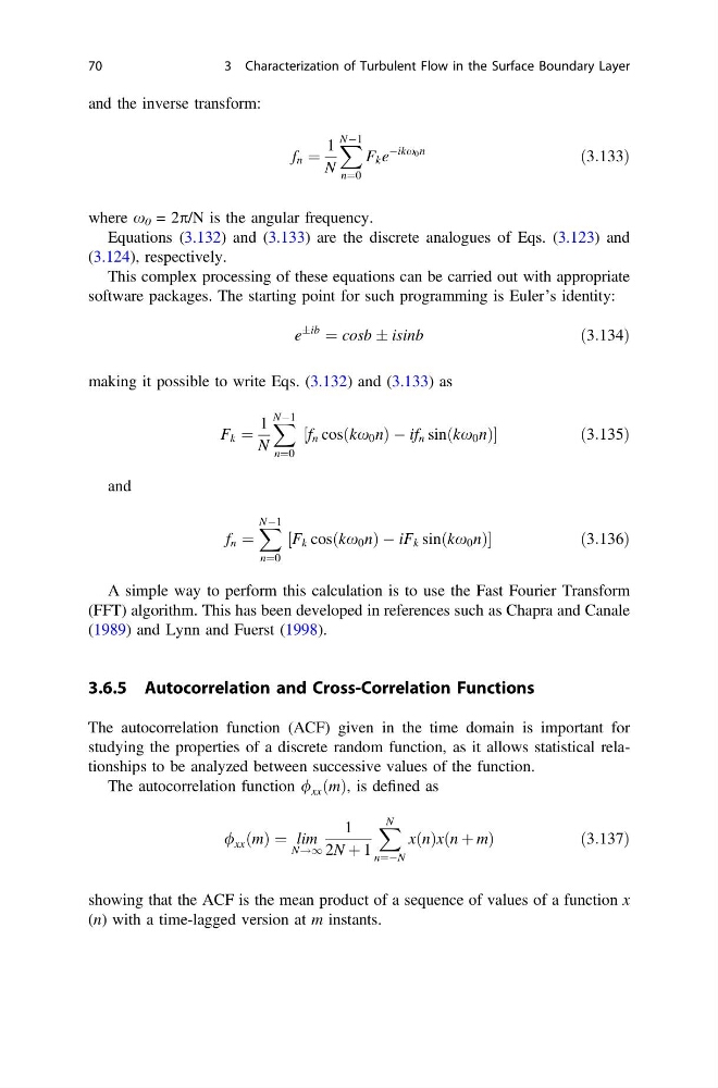
and the inverse transform:
f n ¼
1
N
X NÀ1
n¼0
F k e
Àikx 0 n
ð3:133Þ
where x 0 = 2p/N is the angular frequency.
Equations (3.132) and (3.133) are the discrete analogues of Eqs. (3.123) and
(3.124), respectively.
This complex processing of these equations can be carried out with appropriate
software packages. The starting point for such programming is Euler’s identity:
e
Æib
¼ cosb Æ isinb
ð3:134Þ
making it possible to write Eqs. (3.132) and (3.133) as
F k ¼
1
N
X NÀ1
n¼0
f n cosðkx 0 nÞ À if n sinðkx 0 nÞ
½
ð 3:135Þ
and
f n ¼
X NÀ1
n¼0
F k cosðkx 0 nÞ À iF k sinðkx 0 nÞ
½
ð 3:136Þ
A simple way to perform this calculation is to use the Fast Fourier Transform
(FFT) algorithm. This has been developed in references such as Chapra and Canale
(1989) and Lynn and Fuerst (1998).
3.6.5 Autocorrelation and Cross-Correlation Functions
The autocorrelation function (ACF) given in the time domain is important for
studying the properties of a discrete random function, as it allows statistical relationships to be analyzed between successive values of the function.
The autocorrelation function / xx ðmÞ, is defined as
/ xx ðmÞ ¼ lim
N!1
1
2N þ 1
X N
n¼ÀN
xðnÞxðn þ mÞ
ð 3:137Þ
showing that the ACF is the mean product of a sequence of values of a function x
(n) with a time-lagged version at m instants.
70
3 Characterization of Turbulent Flow in the Surface Boundary Layer
f n ¼
1
N
X NÀ1
n¼0
F k e
Àikx 0 n
ð3:133Þ
where x 0 = 2p/N is the angular frequency.
Equations (3.132) and (3.133) are the discrete analogues of Eqs. (3.123) and
(3.124), respectively.
This complex processing of these equations can be carried out with appropriate
software packages. The starting point for such programming is Euler’s identity:
e
Æib
¼ cosb Æ isinb
ð3:134Þ
making it possible to write Eqs. (3.132) and (3.133) as
F k ¼
1
N
X NÀ1
n¼0
f n cosðkx 0 nÞ À if n sinðkx 0 nÞ
½
ð 3:135Þ
and
f n ¼
X NÀ1
n¼0
F k cosðkx 0 nÞ À iF k sinðkx 0 nÞ
½
ð 3:136Þ
A simple way to perform this calculation is to use the Fast Fourier Transform
(FFT) algorithm. This has been developed in references such as Chapra and Canale
(1989) and Lynn and Fuerst (1998).
3.6.5 Autocorrelation and Cross-Correlation Functions
The autocorrelation function (ACF) given in the time domain is important for
studying the properties of a discrete random function, as it allows statistical relationships to be analyzed between successive values of the function.
The autocorrelation function / xx ðmÞ, is defined as
/ xx ðmÞ ¼ lim
N!1
1
2N þ 1
X N
n¼ÀN
xðnÞxðn þ mÞ
ð 3:137Þ
showing that the ACF is the mean product of a sequence of values of a function x
(n) with a time-lagged version at m instants.
70
3 Characterization of Turbulent Flow in the Surface Boundary Layer