

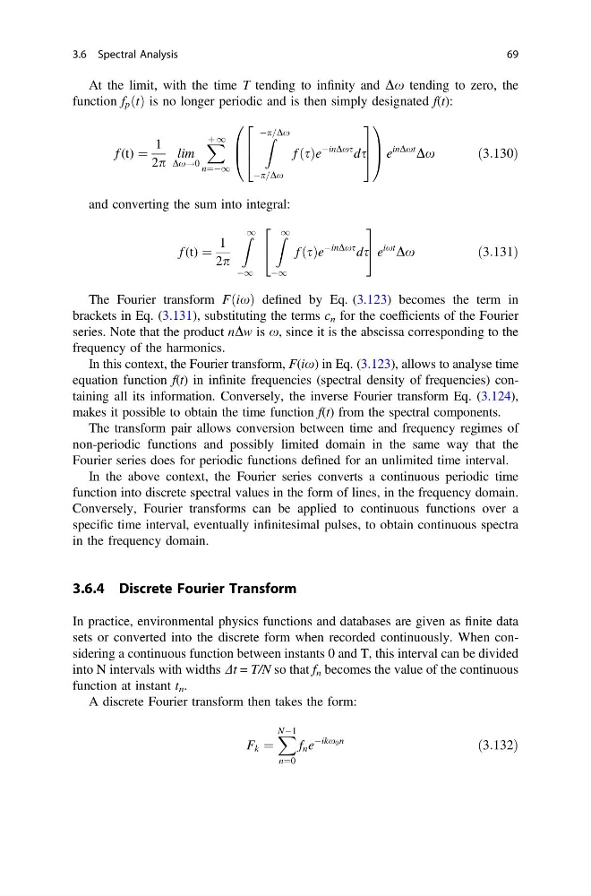
At the limit, with the time T tending to infinity and Dx tending to zero, the
function f p ðtÞ is no longer periodic and is then simply designated f(t):
f (t) ¼
1
2p
lim
Dx!0
X þ 1
n¼À1
Z
Àp=Dx
Àp=Dx
f ðsÞe
ÀinDxs ds
2
6
4
3
7
5
0
B
@
1
C
A e
inDxt
Dx
ð3:130Þ
and converting the sum into integral:
f (t) ¼
1
2p
Z 1
À1
Z 1
À1
f ðsÞe
ÀinDxs ds
2
4
3
5 e
ixt
Dx
ð3:131Þ
The Fourier transform FðixÞ defined by Eq. (3.123) becomes the term in
brackets in Eq. (3.131), substituting the terms c n for the coefficients of the Fourier
series. Note that the product nDw is x, since it is the abscissa corresponding to the
frequency of the harmonics.
In this context, the Fourier transform, F(ix) in Eq. (3.123), allows to analyse time
equation function f(t) in infinite frequencies (spectral density of frequencies) containing all its information. Conversely, the inverse Fourier transform Eq. (3.124),
makes it possible to obtain the time function f(t) from the spectral components.
The transform pair allows conversion between time and frequency regimes of
non-periodic functions and possibly limited domain in the same way that the
Fourier series does for periodic functions defined for an unlimited time interval.
In the above context, the Fourier series converts a continuous periodic time
function into discrete spectral values in the form of lines, in the frequency domain.
Conversely, Fourier transforms can be applied to continuous functions over a
specific time interval, eventually infinitesimal pulses, to obtain continuous spectra
in the frequency domain.
3.6.4 Discrete Fourier Transform
In practice, environmental physics functions and databases are given as finite data
sets or converted into the discrete form when recorded continuously. When considering a continuous function between instants 0 and T, this interval can be divided
into N intervals with widths Dt = T/N so that f n becomes the value of the continuous
function at instant t n .
A discrete Fourier transform then takes the form:
F k ¼
X NÀ1
n¼0
f n e
Àikx 0 n
ð3:132Þ
3.6 Spectral Analysis
69
function f p ðtÞ is no longer periodic and is then simply designated f(t):
f (t) ¼
1
2p
lim
Dx!0
X þ 1
n¼À1
Z
Àp=Dx
Àp=Dx
f ðsÞe
ÀinDxs ds
2
6
4
3
7
5
0
B
@
1
C
A e
inDxt
Dx
ð3:130Þ
and converting the sum into integral:
f (t) ¼
1
2p
Z 1
À1
Z 1
À1
f ðsÞe
ÀinDxs ds
2
4
3
5 e
ixt
Dx
ð3:131Þ
The Fourier transform FðixÞ defined by Eq. (3.123) becomes the term in
brackets in Eq. (3.131), substituting the terms c n for the coefficients of the Fourier
series. Note that the product nDw is x, since it is the abscissa corresponding to the
frequency of the harmonics.
In this context, the Fourier transform, F(ix) in Eq. (3.123), allows to analyse time
equation function f(t) in infinite frequencies (spectral density of frequencies) containing all its information. Conversely, the inverse Fourier transform Eq. (3.124),
makes it possible to obtain the time function f(t) from the spectral components.
The transform pair allows conversion between time and frequency regimes of
non-periodic functions and possibly limited domain in the same way that the
Fourier series does for periodic functions defined for an unlimited time interval.
In the above context, the Fourier series converts a continuous periodic time
function into discrete spectral values in the form of lines, in the frequency domain.
Conversely, Fourier transforms can be applied to continuous functions over a
specific time interval, eventually infinitesimal pulses, to obtain continuous spectra
in the frequency domain.
3.6.4 Discrete Fourier Transform
In practice, environmental physics functions and databases are given as finite data
sets or converted into the discrete form when recorded continuously. When considering a continuous function between instants 0 and T, this interval can be divided
into N intervals with widths Dt = T/N so that f n becomes the value of the continuous
function at instant t n .
A discrete Fourier transform then takes the form:
F k ¼
X NÀ1
n¼0
f n e
Àikx 0 n
ð3:132Þ
3.6 Spectral Analysis
69