

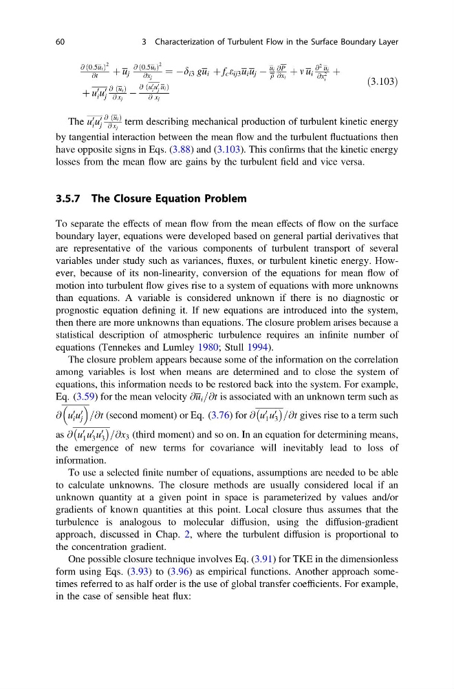
@ 0:5u i
ð
Þ
2
@t
þ u j
@ 0:5u i
ð
Þ
2
@x j
¼ Àd i3 gu i þ f c e ij3 u i u j À
u i
q
@P
@x i
þ m u i
@
2 u i
@x 2
i
þ
þ u 0
i u 0
j
@ ðu i Þ
@ x j
À
@ ðu 0
i u 0
j u i Þ
@ x j
ð3:103Þ
The u 0
i u 0
j
@ ðu i Þ
@ x j
term describing mechanical production of turbulent kinetic energy
by tangential interaction between the mean flow and the turbulent fluctuations then
have opposite signs in Eqs. (3.88) and (3.103). This confirms that the kinetic energy
losses from the mean flow are gains by the turbulent field and vice versa.
3.5.7 The Closure Equation Problem
To separate the effects of mean flow from the mean effects of flow on the surface
boundary layer, equations were developed based on general partial derivatives that
are representative of the various components of turbulent transport of several
variables under study such as variances, fluxes, or turbulent kinetic energy. However, because of its non-linearity, conversion of the equations for mean flow of
motion into turbulent flow gives rise to a system of equations with more unknowns
than equations. A variable is considered unknown if there is no diagnostic or
prognostic equation defining it. If new equations are introduced into the system,
then there are more unknowns than equations. The closure problem arises because a
statistical description of atmospheric turbulence requires an infinite number of
equations (Tennekes and Lumley 1980; Stull 1994).
The closure problem appears because some of the information on the correlation
among variables is lost when means are determined and to close the system of
equations, this information needs to be restored back into the system. For example,
Eq. (3.59) for the mean velocity @u i =@t is associated with an unknown term such as
@ u 0
i u 0
j
=@t (second moment) or Eq. (3.76) for @ u 0
1 u 0
3
À
Á =@t gives rise to a term such
as @ u 0
1 u 0
3 u 0
3
À
Á =@x 3 (third moment) and so on. In an equation for determining means,
the emergence of new terms for covariance will inevitably lead to loss of
information.
To use a selected finite number of equations, assumptions are needed to be able
to calculate unknowns. The closure methods are usually considered local if an
unknown quantity at a given point in space is parameterized by values and/or
gradients of known quantities at this point. Local closure thus assumes that the
turbulence is analogous to molecular diffusion, using the diffusion-gradient
approach, discussed in Chap. 2, where the turbulent diffusion is proportional to
the concentration gradient.
One possible closure technique involves Eq. (3.91) for TKE in the dimensionless
form using Eqs. (3.93) to (3.96) as empirical functions. Another approach sometimes referred to as half order is the use of global transfer coefficients. For example,
in the case of sensible heat flux:
60
3 Characterization of Turbulent Flow in the Surface Boundary Layer
ð
Þ
2
@t
þ u j
@ 0:5u i
ð
Þ
2
@x j
¼ Àd i3 gu i þ f c e ij3 u i u j À
u i
q
@P
@x i
þ m u i
@
2 u i
@x 2
i
þ
þ u 0
i u 0
j
@ ðu i Þ
@ x j
À
@ ðu 0
i u 0
j u i Þ
@ x j
ð3:103Þ
The u 0
i u 0
j
@ ðu i Þ
@ x j
term describing mechanical production of turbulent kinetic energy
by tangential interaction between the mean flow and the turbulent fluctuations then
have opposite signs in Eqs. (3.88) and (3.103). This confirms that the kinetic energy
losses from the mean flow are gains by the turbulent field and vice versa.
3.5.7 The Closure Equation Problem
To separate the effects of mean flow from the mean effects of flow on the surface
boundary layer, equations were developed based on general partial derivatives that
are representative of the various components of turbulent transport of several
variables under study such as variances, fluxes, or turbulent kinetic energy. However, because of its non-linearity, conversion of the equations for mean flow of
motion into turbulent flow gives rise to a system of equations with more unknowns
than equations. A variable is considered unknown if there is no diagnostic or
prognostic equation defining it. If new equations are introduced into the system,
then there are more unknowns than equations. The closure problem arises because a
statistical description of atmospheric turbulence requires an infinite number of
equations (Tennekes and Lumley 1980; Stull 1994).
The closure problem appears because some of the information on the correlation
among variables is lost when means are determined and to close the system of
equations, this information needs to be restored back into the system. For example,
Eq. (3.59) for the mean velocity @u i =@t is associated with an unknown term such as
@ u 0
i u 0
j
=@t (second moment) or Eq. (3.76) for @ u 0
1 u 0
3
À
Á =@t gives rise to a term such
as @ u 0
1 u 0
3 u 0
3
À
Á =@x 3 (third moment) and so on. In an equation for determining means,
the emergence of new terms for covariance will inevitably lead to loss of
information.
To use a selected finite number of equations, assumptions are needed to be able
to calculate unknowns. The closure methods are usually considered local if an
unknown quantity at a given point in space is parameterized by values and/or
gradients of known quantities at this point. Local closure thus assumes that the
turbulence is analogous to molecular diffusion, using the diffusion-gradient
approach, discussed in Chap. 2, where the turbulent diffusion is proportional to
the concentration gradient.
One possible closure technique involves Eq. (3.91) for TKE in the dimensionless
form using Eqs. (3.93) to (3.96) as empirical functions. Another approach sometimes referred to as half order is the use of global transfer coefficients. For example,
in the case of sensible heat flux:
60
3 Characterization of Turbulent Flow in the Surface Boundary Layer