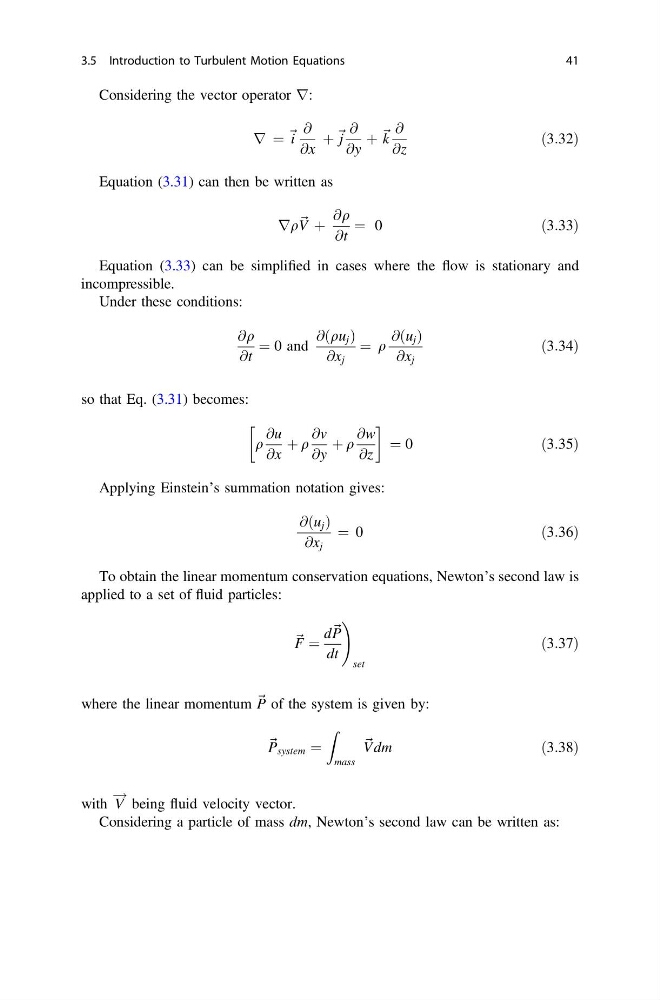
Considering the vector operator r:
r ¼ ~ i
@
@x
þ ~ j
@
@y
þ ~ k
@
@z
ð3:32Þ
Equation (3.31) can then be written as
rq ~ V þ
@q
@t
¼ 0
ð3:33Þ
Equation (3.33) can be simplified in cases where the flow is stationary and
incompressible.
Under these conditions:
@q
@t
¼ 0 and
@ðqu j Þ
@x j
¼ q
@ðu j Þ
@x j
ð3:34Þ
so that Eq. (3.31) becomes:
q
@u
@x
þ q
@v
@y
þ q
@w
@z
!
¼ 0
ð3:35Þ
Applying Einstein’s summation notation gives:
@ðu j Þ
@x j
¼ 0
ð3:36Þ
To obtain the linear momentum conservation equations, Newton’s second law is
applied to a set of fluid particles:
~ F ¼
d ~ P
dt
!
set
ð3:37Þ
where the linear momentum ~ P of the system is given by:
~ P system ¼
Z
mass
~ Vdm
ð3:38Þ
with V
! being fluid velocity vector.
Considering a particle of mass dm, Newton’s second law can be written as:
3.5 Introduction to Turbulent Motion Equations
41