

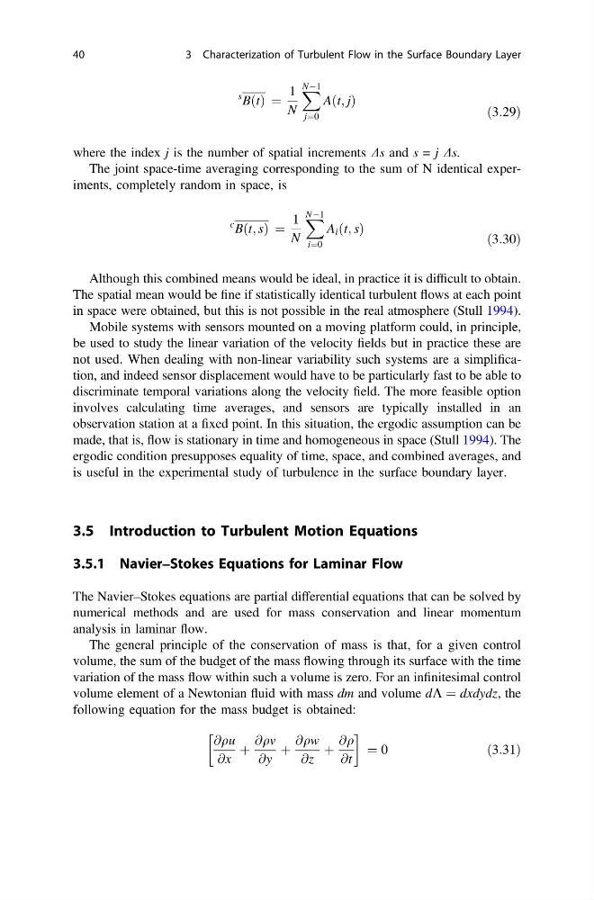
s BðtÞ ¼
1
N
X NÀ1
j¼0
Aðt; jÞ
ð3:29Þ
where the index j is the number of spatial increments Ds and s = j Ds.
The joint space-time averaging corresponding to the sum of N identical experiments, completely random in space, is
c Bðt; sÞ ¼
1
N
X NÀ1
i¼0
A i ðt; sÞ
ð3:30Þ
Although this combined means would be ideal, in practice it is difficult to obtain.
The spatial mean would be fine if statistically identical turbulent flows at each point
in space were obtained, but this is not possible in the real atmosphere (Stull 1994).
Mobile systems with sensors mounted on a moving platform could, in principle,
be used to study the linear variation of the velocity fields but in practice these are
not used. When dealing with non-linear variability such systems are a simplification, and indeed sensor displacement would have to be particularly fast to be able to
discriminate temporal variations along the velocity field. The more feasible option
involves calculating time averages, and sensors are typically installed in an
observation station at a fixed point. In this situation, the ergodic assumption can be
made, that is, flow is stationary in time and homogeneous in space (Stull 1994). The
ergodic condition presupposes equality of time, space, and combined averages, and
is useful in the experimental study of turbulence in the surface boundary layer.
3.5 Introduction to Turbulent Motion Equations
3.5.1 Navier–Stokes Equations for Laminar Flow
The Navier–Stokes equations are partial differential equations that can be solved by
numerical methods and are used for mass conservation and linear momentum
analysis in laminar flow.
The general principle of the conservation of mass is that, for a given control
volume, the sum of the budget of the mass flowing through its surface with the time
variation of the mass flow within such a volume is zero. For an infinitesimal control
volume element of a Newtonian fluid with mass dm and volume dK ¼ dxdydz, the
following equation for the mass budget is obtained:
@qu
@x
þ
@qv
@y
þ
@qw
@z
þ
@q
@t
!
¼ 0
ð3:31Þ
40
3 Characterization of Turbulent Flow in the Surface Boundary Layer
1
N
X NÀ1
j¼0
Aðt; jÞ
ð3:29Þ
where the index j is the number of spatial increments Ds and s = j Ds.
The joint space-time averaging corresponding to the sum of N identical experiments, completely random in space, is
c Bðt; sÞ ¼
1
N
X NÀ1
i¼0
A i ðt; sÞ
ð3:30Þ
Although this combined means would be ideal, in practice it is difficult to obtain.
The spatial mean would be fine if statistically identical turbulent flows at each point
in space were obtained, but this is not possible in the real atmosphere (Stull 1994).
Mobile systems with sensors mounted on a moving platform could, in principle,
be used to study the linear variation of the velocity fields but in practice these are
not used. When dealing with non-linear variability such systems are a simplification, and indeed sensor displacement would have to be particularly fast to be able to
discriminate temporal variations along the velocity field. The more feasible option
involves calculating time averages, and sensors are typically installed in an
observation station at a fixed point. In this situation, the ergodic assumption can be
made, that is, flow is stationary in time and homogeneous in space (Stull 1994). The
ergodic condition presupposes equality of time, space, and combined averages, and
is useful in the experimental study of turbulence in the surface boundary layer.
3.5 Introduction to Turbulent Motion Equations
3.5.1 Navier–Stokes Equations for Laminar Flow
The Navier–Stokes equations are partial differential equations that can be solved by
numerical methods and are used for mass conservation and linear momentum
analysis in laminar flow.
The general principle of the conservation of mass is that, for a given control
volume, the sum of the budget of the mass flowing through its surface with the time
variation of the mass flow within such a volume is zero. For an infinitesimal control
volume element of a Newtonian fluid with mass dm and volume dK ¼ dxdydz, the
following equation for the mass budget is obtained:
@qu
@x
þ
@qv
@y
þ
@qw
@z
þ
@q
@t
!
¼ 0
ð3:31Þ
40
3 Characterization of Turbulent Flow in the Surface Boundary Layer