

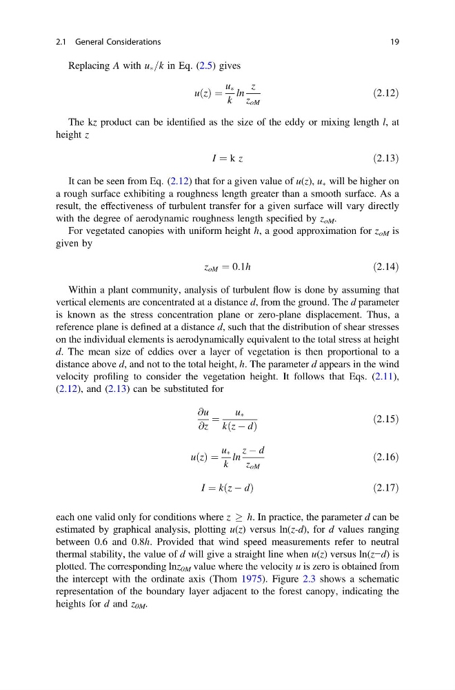
Replacing A with u à =k in Eq. (2.5) gives
u z
ð Þ ¼
u Ã
k
ln
z
z oM
ð2:12Þ
The kz product can be identified as the size of the eddy or mixing length l, at
height z
I ¼ k z
ð2:13Þ
It can be seen from Eq. (2.12) that for a given value of u(z), u à will be higher on
a rough surface exhibiting a roughness length greater than a smooth surface. As a
result, the effectiveness of turbulent transfer for a given surface will vary directly
with the degree of aerodynamic roughness length specified by z oM .
For vegetated canopies with uniform height h, a good approximation for z oM is
given by
z oM ¼ 0:1h
ð2:14Þ
Within a plant community, analysis of turbulent flow is done by assuming that
vertical elements are concentrated at a distance d, from the ground. The d parameter
is known as the stress concentration plane or zero-plane displacement. Thus, a
reference plane is defined at a distance d, such that the distribution of shear stresses
on the individual elements is aerodynamically equivalent to the total stress at height
d. The mean size of eddies over a layer of vegetation is then proportional to a
distance above d, and not to the total height, h. The parameter d appears in the wind
velocity profiling to consider the vegetation height. It follows that Eqs. (2.11),
(2.12), and (2.13) can be substituted for
@u
@z
¼
u Ã
k z À d
ð
Þ
ð2:15Þ
u z
ð Þ ¼
u Ã
k
ln
z À d
z oM
ð2:16Þ
I ¼ kðz À dÞ
ð 2:17Þ
each one valid only for conditions where z ! h. In practice, the parameter d can be
estimated by graphical analysis, plotting u(z) versus ln(z-d), for d values ranging
between 0.6 and 0.8h. Provided that wind speed measurements refer to neutral
thermal stability, the value of d will give a straight line when u(z) versus ln(z−d) is
plotted. The corresponding lnz 0M value where the velocity u is zero is obtained from
the intercept with the ordinate axis (Thom 1975). Figure 2.3 shows a schematic
representation of the boundary layer adjacent to the forest canopy, indicating the
heights for d and z 0M .
2.1 General Considerations
19
u z
ð Þ ¼
u Ã
k
ln
z
z oM
ð2:12Þ
The kz product can be identified as the size of the eddy or mixing length l, at
height z
I ¼ k z
ð2:13Þ
It can be seen from Eq. (2.12) that for a given value of u(z), u à will be higher on
a rough surface exhibiting a roughness length greater than a smooth surface. As a
result, the effectiveness of turbulent transfer for a given surface will vary directly
with the degree of aerodynamic roughness length specified by z oM .
For vegetated canopies with uniform height h, a good approximation for z oM is
given by
z oM ¼ 0:1h
ð2:14Þ
Within a plant community, analysis of turbulent flow is done by assuming that
vertical elements are concentrated at a distance d, from the ground. The d parameter
is known as the stress concentration plane or zero-plane displacement. Thus, a
reference plane is defined at a distance d, such that the distribution of shear stresses
on the individual elements is aerodynamically equivalent to the total stress at height
d. The mean size of eddies over a layer of vegetation is then proportional to a
distance above d, and not to the total height, h. The parameter d appears in the wind
velocity profiling to consider the vegetation height. It follows that Eqs. (2.11),
(2.12), and (2.13) can be substituted for
@u
@z
¼
u Ã
k z À d
ð
Þ
ð2:15Þ
u z
ð Þ ¼
u Ã
k
ln
z À d
z oM
ð2:16Þ
I ¼ kðz À dÞ
ð 2:17Þ
each one valid only for conditions where z ! h. In practice, the parameter d can be
estimated by graphical analysis, plotting u(z) versus ln(z-d), for d values ranging
between 0.6 and 0.8h. Provided that wind speed measurements refer to neutral
thermal stability, the value of d will give a straight line when u(z) versus ln(z−d) is
plotted. The corresponding lnz 0M value where the velocity u is zero is obtained from
the intercept with the ordinate axis (Thom 1975). Figure 2.3 shows a schematic
representation of the boundary layer adjacent to the forest canopy, indicating the
heights for d and z 0M .
2.1 General Considerations
19