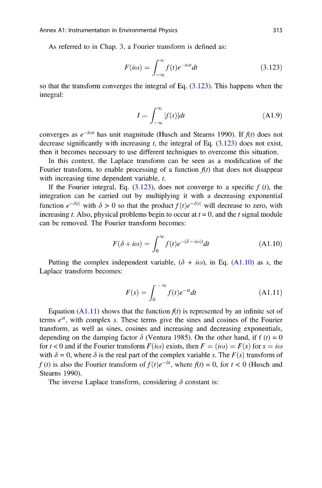
As referred to in Chap. 3, a Fourier transform is defined as:
FðixÞ ¼
Z 1
À1
f ðtÞe
Àixt dt
ð3:123Þ
so that the transform converges the integral of Eq. (3.123). This happens when the
integral:
I ¼
Z 1
À1
jf ðtÞjdt
ðA1:9Þ
converges as e
Àixt has unit magnitude (Husch and Stearns 1990). If f(t) does not
decrease significantly with increasing t, the integral of Eq. (3.123) does not exist,
then it becomes necessary to use different techniques to overcome this situation.
In this context, the Laplace transform can be seen as a modification of the
Fourier transform, to enable processing of a function f(t) that does not disappear
with increasing time dependent variable, t.
If the Fourier integral, Eq. (3.123), does not converge to a specific f (t), the
integration can be carried out by multiplying it with a decreasing exponential
function e
Àd t
j j with d > 0 so that the product f ðtÞe
Àd t
j j will decrease to zero, with
increasing t. Also, physical problems begin to occur at t = 0, and the t signal module
can be removed. The Fourier transform becomes:
Fðd þ ixÞ ¼
Z 1
0
f ðtÞe
Àðd þ ixÞt dt
ðA1:10Þ
Putting the complex independent variable, (d + ix), in Eq. (A1.10) as s, the
Laplace transform becomes:
FðsÞ ¼
Z þ 1
0
f ðtÞe
Àst dt
ðA1:11Þ
Equation (A1.11) shows that the function f(t) is represented by an infinite set of
terms e
st
; with complex s. These terms give the sines and cosines of the Fourier
transform, as well as sines, cosines and increasing and decreasing exponentials,
depending on the damping factor d (Ventura 1985). On the other hand, if f (t) = 0
for t < 0 and if the Fourier transform F ix
ð Þ exists, then F ¼ ix
ð Þ ¼ FðsÞ for s ¼ ix
with d = 0, where d is the real part of the complex variable s. The FðsÞ transform of
f (t) is also the Fourier transform of f ðtÞe
Àdt , where f(t) = 0, for t < 0 (Husch and
Stearns 1990).
The inverse Laplace transform, considering d constant is:
Annex A1: Instrumentation in Environmental Physics
315