

f ðtÞ ¼
1
2p i
Z
d þ i1
dÀi1
FðsÞe
st ds
ðA1:12Þ
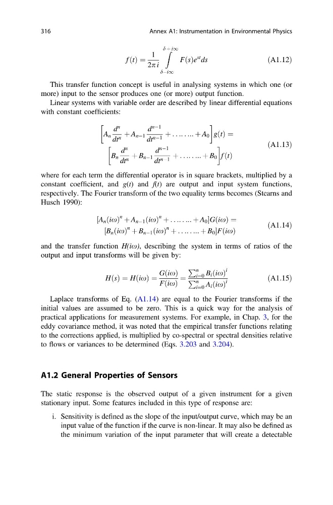
This transfer function concept is useful in analysing systems in which one (or
more) input to the sensor produces one (or more) output function.
Linear systems with variable order are described by linear differential equations
with constant coefficients:
A n
d
n
dt n þ A nÀ1
d
nÀ1
dt nÀ1 þ . . .. . .:: þ A 0
!
gðtÞ ¼
B n
d
n
dt n þ B nÀ1
d
nÀ1
dt nÀ1 þ . . .. . .:: þ B 0
!
f ðtÞ
ðA1:13Þ
where for each term the differential operator is in square brackets, multiplied by a
constant coefficient, and g(t) and f(t) are output and input system functions,
respectively. The Fourier transform of the two equality terms becomes (Stearns and
Husch 1990):
A n ix
ð Þ
n þ A nÀ1 ix
ð Þ
n þ . . .. . .:: þ A 0
½
GðixÞ ¼
B n ix
ð Þ
n þ B nÀ1 ix
ð Þ
n þ . . .. . .:: þ B 0
½
FðixÞ
ðA1:14Þ
and the transfer function H(ix), describing the system in terms of ratios of the
output and input transforms will be given by:
HðsÞ ¼ HðixÞ ¼
GðixÞ
FðixÞ
¼
P n
i¼0 B i ðixÞ
i
P n
i¼0 A i ðixÞ
i
ðA1:15Þ
Laplace transforms of Eq. (A1.14) are equal to the Fourier transforms if the
initial values are assumed to be zero. This is a quick way for the analysis of
practical applications for measurement systems. For example, in Chap. 3, for the
eddy covariance method, it was noted that the empirical transfer functions relating
to the corrections applied, is multiplied by co-spectral or spectral densities relative
to flows or variances to be determined (Eqs. 3.203 and 3.204).
A1.2 General Properties of Sensors
The static response is the observed output of a given instrument for a given
stationary input. Some features included in this type of response are:
i. Sensitivity is defined as the slope of the input/output curve, which may be an
input value of the function if the curve is non-linear. It may also be defined as
the minimum variation of the input parameter that will create a detectable
316
Annex A1: Instrumentation in Environmental Physics
1
2p i
Z
d þ i1
dÀi1
FðsÞe
st ds
ðA1:12Þ
This transfer function concept is useful in analysing systems in which one (or
more) input to the sensor produces one (or more) output function.
Linear systems with variable order are described by linear differential equations
with constant coefficients:
A n
d
n
dt n þ A nÀ1
d
nÀ1
dt nÀ1 þ . . .. . .:: þ A 0
!
gðtÞ ¼
B n
d
n
dt n þ B nÀ1
d
nÀ1
dt nÀ1 þ . . .. . .:: þ B 0
!
f ðtÞ
ðA1:13Þ
where for each term the differential operator is in square brackets, multiplied by a
constant coefficient, and g(t) and f(t) are output and input system functions,
respectively. The Fourier transform of the two equality terms becomes (Stearns and
Husch 1990):
A n ix
ð Þ
n þ A nÀ1 ix
ð Þ
n þ . . .. . .:: þ A 0
½
GðixÞ ¼
B n ix
ð Þ
n þ B nÀ1 ix
ð Þ
n þ . . .. . .:: þ B 0
½
FðixÞ
ðA1:14Þ
and the transfer function H(ix), describing the system in terms of ratios of the
output and input transforms will be given by:
HðsÞ ¼ HðixÞ ¼
GðixÞ
FðixÞ
¼
P n
i¼0 B i ðixÞ
i
P n
i¼0 A i ðixÞ
i
ðA1:15Þ
Laplace transforms of Eq. (A1.14) are equal to the Fourier transforms if the
initial values are assumed to be zero. This is a quick way for the analysis of
practical applications for measurement systems. For example, in Chap. 3, for the
eddy covariance method, it was noted that the empirical transfer functions relating
to the corrections applied, is multiplied by co-spectral or spectral densities relative
to flows or variances to be determined (Eqs. 3.203 and 3.204).
A1.2 General Properties of Sensors
The static response is the observed output of a given instrument for a given
stationary input. Some features included in this type of response are:
i. Sensitivity is defined as the slope of the input/output curve, which may be an
input value of the function if the curve is non-linear. It may also be defined as
the minimum variation of the input parameter that will create a detectable
316
Annex A1: Instrumentation in Environmental Physics