

yðtÞ ¼ K½1 À ð1 þ xtÞexpðÀxtÞ
ðA1:8Þ
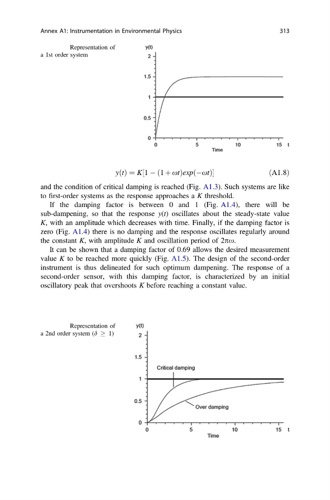
and the condition of critical damping is reached (Fig. A1.3). Such systems are like
to first-order systems as the response approaches a K threshold.
If the damping factor is between 0 and 1 (Fig. A1.4), there will be
sub-dampening, so that the response y(t) oscillates about the steady-state value
K, with an amplitude which decreases with time. Finally, if the damping factor is
zero (Fig. A1.4) there is no damping and the response oscillates regularly around
the constant K, with amplitude K and oscillation period of 2px.
It can be shown that a damping factor of 0.69 allows the desired measurement
value K to be reached more quickly (Fig. A1.5). The design of the second-order
instrument is thus delineated for such optimum dampening. The response of a
second-order sensor, with this damping factor, is characterized by an initial
oscillatory peak that overshoots K before reaching a constant value.
Fig. A1.2 Representation of
a 1st order system
Fig. A1.3 Representation of
a 2nd order system (d ! 1)
Annex A1: Instrumentation in Environmental Physics
313
ðA1:8Þ
and the condition of critical damping is reached (Fig. A1.3). Such systems are like
to first-order systems as the response approaches a K threshold.
If the damping factor is between 0 and 1 (Fig. A1.4), there will be
sub-dampening, so that the response y(t) oscillates about the steady-state value
K, with an amplitude which decreases with time. Finally, if the damping factor is
zero (Fig. A1.4) there is no damping and the response oscillates regularly around
the constant K, with amplitude K and oscillation period of 2px.
It can be shown that a damping factor of 0.69 allows the desired measurement
value K to be reached more quickly (Fig. A1.5). The design of the second-order
instrument is thus delineated for such optimum dampening. The response of a
second-order sensor, with this damping factor, is characterized by an initial
oscillatory peak that overshoots K before reaching a constant value.
Fig. A1.2 Representation of
a 1st order system
Fig. A1.3 Representation of
a 2nd order system (d ! 1)
Annex A1: Instrumentation in Environmental Physics
313