

opposes these natural fluctuations, with intensity proportional to the rate of change
of output signal. The damping factor is a measure of the opposition to the natural
oscillations. Depending on the extent of damping, a second-order system can
stabilize in the form of undampened oscillations when subjected to input in the form
of a step function. Wind direction sensors are an example of such systems.
If the input function x(t) varies continuously with time, the output of a zero-order
apparatus varies the same way, being multiplied by a static gain k. Conversely,
outputs of first and second-order instruments do not vary in the same way. In these
instruments, the configuration of the output function y(t), is different from that of
the input function x(t).
It follows from the above that the response of various systems (zero, one or two
order) to a step function, characterized by a quick change in the input value such as
x(t) = 0 for t
0 and x(t) = 1 for t > 0 is:
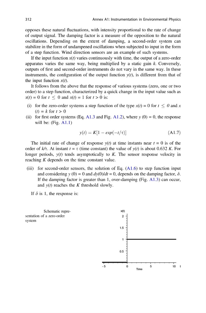
(i) for the zero-order systems a step function of the type x(t) = 0 for t
0 and x
(t) = k for t > 0
(ii) for first order systems (Eq. A1.3 and Fig. A1.2), where y (0) = 0, the response
will be: (Fig. A1.1)
yðtÞ ¼ K½1 À expðÀt=sÞ
ðA1:7Þ
The initial rate of change of response y(t) at time instants near t = 0 is of the
order of k/s. At instant t = s (time constant) the value of y(t) is about 0.632 K. For
longer periods, y(t) tends asymptotically to K. The sensor response velocity in
reaching K depends on the time constant value.
(iii) for second-order sensors, the solution of Eq. (A1.6) to step function input
and considering y (0) = 0 and dy(0)/dt = 0, depends on the damping factor, d.
If the damping factor is greater than 1, over-damping (Fig. A1.3) can occur,
and y(t) reaches the K threshold slowly.
If d is 1, the response is:
Fig. A1.1 Schematic representation of a zero-order
system
312
Annex A1: Instrumentation in Environmental Physics
of output signal. The damping factor is a measure of the opposition to the natural
oscillations. Depending on the extent of damping, a second-order system can
stabilize in the form of undampened oscillations when subjected to input in the form
of a step function. Wind direction sensors are an example of such systems.
If the input function x(t) varies continuously with time, the output of a zero-order
apparatus varies the same way, being multiplied by a static gain k. Conversely,
outputs of first and second-order instruments do not vary in the same way. In these
instruments, the configuration of the output function y(t), is different from that of
the input function x(t).
It follows from the above that the response of various systems (zero, one or two
order) to a step function, characterized by a quick change in the input value such as
x(t) = 0 for t
0 and x(t) = 1 for t > 0 is:
(i) for the zero-order systems a step function of the type x(t) = 0 for t
0 and x
(t) = k for t > 0
(ii) for first order systems (Eq. A1.3 and Fig. A1.2), where y (0) = 0, the response
will be: (Fig. A1.1)
yðtÞ ¼ K½1 À expðÀt=sÞ
ðA1:7Þ
The initial rate of change of response y(t) at time instants near t = 0 is of the
order of k/s. At instant t = s (time constant) the value of y(t) is about 0.632 K. For
longer periods, y(t) tends asymptotically to K. The sensor response velocity in
reaching K depends on the time constant value.
(iii) for second-order sensors, the solution of Eq. (A1.6) to step function input
and considering y (0) = 0 and dy(0)/dt = 0, depends on the damping factor, d.
If the damping factor is greater than 1, over-damping (Fig. A1.3) can occur,
and y(t) reaches the K threshold slowly.
If d is 1, the response is:
Fig. A1.1 Schematic representation of a zero-order
system
312
Annex A1: Instrumentation in Environmental Physics