

stability and a bit higher (0.8–1) under thermal instability conditions. The parameter
c, is about 0.2–0.8, being higher under thermal instability and lower under thermal
stability conditions.
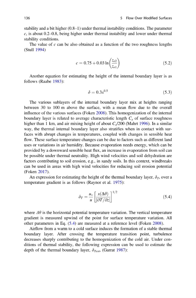
The value of c can be also obtained as a function of the two roughness lengths
(Stull 1994)
c ¼ 0:75 þ 0:03 ln
z o2
z o1
ð5:2Þ
Another equation for estimating the height of the internal boundary layer is as
follows (Raabe 1983):
d ¼ 0:3x
0:5
ð5:3Þ
The various sublayers of the internal boundary layer mix at heights ranging
between 30 to 100 m above the surface, with a mean flow due to the overall
influence of the various surfaces (Foken 2008). This homogenization of the internal
boundary layer is related to average characteristic length C x of surface roughness
higher than 1 km, and air mixing height of about C x /200 (Mahrt 1996). In a similar
way, the thermal internal boundary layer also stratifies when in contact with surfaces with abrupt changes in temperatures, coupled with changes in sensible heat
flow. These surface temperature changes can be due to factors such as different land
uses or variations in air humidity. Because evaporation needs energy, which can be
provided by a downward sensible heat flux, an increase in evaporation from soil can
be possible under thermal neutrality. High wind velocities and soil dehydration are
factors contributing to soil erosion, e.g., in sandy soils. In this context, windbreaks
can be used in areas with high wind velocities for reducing soil erosion potential
(Foken 2017).
An expression for estimating the height of the thermal boundary layer, d T , over a
temperature gradient is as follows (Raynor et al. 1975):
d T ¼
u Ã
u
xðDhÞ
@T=@z
j
j
1=2
ð5:4Þ
where Dh is the horizontal potential temperature variation. The vertical temperature
gradient is measured upwind of the point for surface temperature variation. All
other parameters in Eq. (5.4) are measured at a reference level (Foken 2008).
Airflow from a warm to a cold surface induces the formation of a stable thermal
boundary layer. After crossing the temperature transition point, turbulence
decreases sharply contributing to the homogenization of the cold air. Under conditions of thermal stability, the following expression can be used to estimate the
depth of the thermal boundary layer, d Test , (Garrat 1987):
136
5 Flow Over Modified Surfaces
c, is about 0.2–0.8, being higher under thermal instability and lower under thermal
stability conditions.
The value of c can be also obtained as a function of the two roughness lengths
(Stull 1994)
c ¼ 0:75 þ 0:03 ln
z o2
z o1
ð5:2Þ
Another equation for estimating the height of the internal boundary layer is as
follows (Raabe 1983):
d ¼ 0:3x
0:5
ð5:3Þ
The various sublayers of the internal boundary layer mix at heights ranging
between 30 to 100 m above the surface, with a mean flow due to the overall
influence of the various surfaces (Foken 2008). This homogenization of the internal
boundary layer is related to average characteristic length C x of surface roughness
higher than 1 km, and air mixing height of about C x /200 (Mahrt 1996). In a similar
way, the thermal internal boundary layer also stratifies when in contact with surfaces with abrupt changes in temperatures, coupled with changes in sensible heat
flow. These surface temperature changes can be due to factors such as different land
uses or variations in air humidity. Because evaporation needs energy, which can be
provided by a downward sensible heat flux, an increase in evaporation from soil can
be possible under thermal neutrality. High wind velocities and soil dehydration are
factors contributing to soil erosion, e.g., in sandy soils. In this context, windbreaks
can be used in areas with high wind velocities for reducing soil erosion potential
(Foken 2017).
An expression for estimating the height of the thermal boundary layer, d T , over a
temperature gradient is as follows (Raynor et al. 1975):
d T ¼
u Ã
u
xðDhÞ
@T=@z
j
j
1=2
ð5:4Þ
where Dh is the horizontal potential temperature variation. The vertical temperature
gradient is measured upwind of the point for surface temperature variation. All
other parameters in Eq. (5.4) are measured at a reference level (Foken 2008).
Airflow from a warm to a cold surface induces the formation of a stable thermal
boundary layer. After crossing the temperature transition point, turbulence
decreases sharply contributing to the homogenization of the cold air. Under conditions of thermal stability, the following expression can be used to estimate the
depth of the thermal boundary layer, d Test , (Garrat 1987):
136
5 Flow Over Modified Surfaces