

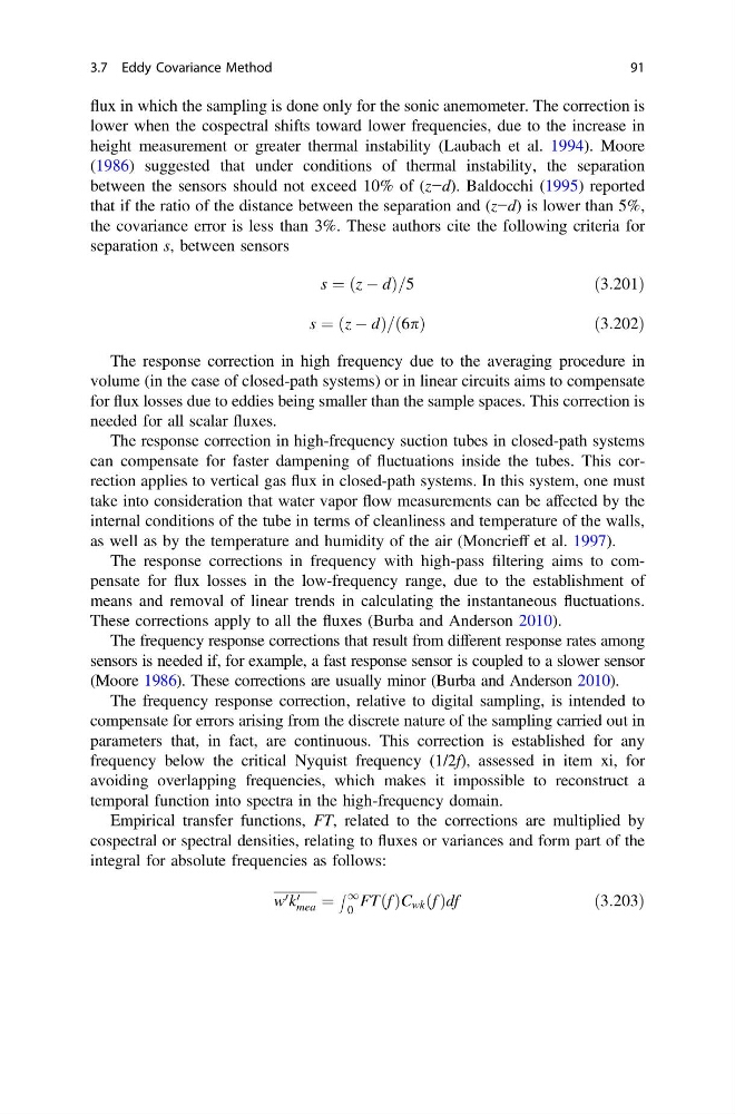
flux in which the sampling is done only for the sonic anemometer. The correction is
lower when the cospectral shifts toward lower frequencies, due to the increase in
height measurement or greater thermal instability (Laubach et al. 1994). Moore
(1986) suggested that under conditions of thermal instability, the separation
between the sensors should not exceed 10% of (z−d). Baldocchi (1995) reported
that if the ratio of the distance between the separation and (z−d) is lower than 5%,
the covariance error is less than 3%. These authors cite the following criteria for
separation s, between sensors
s ¼ ðz À dÞ=5
ð3:201Þ
s ¼ ðz À dÞ=ð6pÞ
ð 3:202Þ
The response correction in high frequency due to the averaging procedure in
volume (in the case of closed-path systems) or in linear circuits aims to compensate
for flux losses due to eddies being smaller than the sample spaces. This correction is
needed for all scalar fluxes.
The response correction in high-frequency suction tubes in closed-path systems
can compensate for faster dampening of fluctuations inside the tubes. This correction applies to vertical gas flux in closed-path systems. In this system, one must
take into consideration that water vapor flow measurements can be affected by the
internal conditions of the tube in terms of cleanliness and temperature of the walls,
as well as by the temperature and humidity of the air (Moncrieff et al. 1997).
The response corrections in frequency with high-pass filtering aims to compensate for flux losses in the low-frequency range, due to the establishment of
means and removal of linear trends in calculating the instantaneous fluctuations.
These corrections apply to all the fluxes (Burba and Anderson 2010).
The frequency response corrections that result from different response rates among
sensors is needed if, for example, a fast response sensor is coupled to a slower sensor
(Moore 1986). These corrections are usually minor (Burba and Anderson 2010).
The frequency response correction, relative to digital sampling, is intended to
compensate for errors arising from the discrete nature of the sampling carried out in
parameters that, in fact, are continuous. This correction is established for any
frequency below the critical Nyquist frequency (1/2f), assessed in item xi, for
avoiding overlapping frequencies, which makes it impossible to reconstruct a
temporal function into spectra in the high-frequency domain.
Empirical transfer functions, FT, related to the corrections are multiplied by
cospectral or spectral densities, relating to fluxes or variances and form part of the
integral for absolute frequencies as follows:
w 0 k 0
mea ¼
Z 1
0
FTðf ÞC wk ðf Þdf
ð3:203Þ
3.7 Eddy Covariance Method
91
lower when the cospectral shifts toward lower frequencies, due to the increase in
height measurement or greater thermal instability (Laubach et al. 1994). Moore
(1986) suggested that under conditions of thermal instability, the separation
between the sensors should not exceed 10% of (z−d). Baldocchi (1995) reported
that if the ratio of the distance between the separation and (z−d) is lower than 5%,
the covariance error is less than 3%. These authors cite the following criteria for
separation s, between sensors
s ¼ ðz À dÞ=5
ð3:201Þ
s ¼ ðz À dÞ=ð6pÞ
ð 3:202Þ
The response correction in high frequency due to the averaging procedure in
volume (in the case of closed-path systems) or in linear circuits aims to compensate
for flux losses due to eddies being smaller than the sample spaces. This correction is
needed for all scalar fluxes.
The response correction in high-frequency suction tubes in closed-path systems
can compensate for faster dampening of fluctuations inside the tubes. This correction applies to vertical gas flux in closed-path systems. In this system, one must
take into consideration that water vapor flow measurements can be affected by the
internal conditions of the tube in terms of cleanliness and temperature of the walls,
as well as by the temperature and humidity of the air (Moncrieff et al. 1997).
The response corrections in frequency with high-pass filtering aims to compensate for flux losses in the low-frequency range, due to the establishment of
means and removal of linear trends in calculating the instantaneous fluctuations.
These corrections apply to all the fluxes (Burba and Anderson 2010).
The frequency response corrections that result from different response rates among
sensors is needed if, for example, a fast response sensor is coupled to a slower sensor
(Moore 1986). These corrections are usually minor (Burba and Anderson 2010).
The frequency response correction, relative to digital sampling, is intended to
compensate for errors arising from the discrete nature of the sampling carried out in
parameters that, in fact, are continuous. This correction is established for any
frequency below the critical Nyquist frequency (1/2f), assessed in item xi, for
avoiding overlapping frequencies, which makes it impossible to reconstruct a
temporal function into spectra in the high-frequency domain.
Empirical transfer functions, FT, related to the corrections are multiplied by
cospectral or spectral densities, relating to fluxes or variances and form part of the
integral for absolute frequencies as follows:
w 0 k 0
mea ¼
Z 1
0
FTðf ÞC wk ðf Þdf
ð3:203Þ
3.7 Eddy Covariance Method
91