

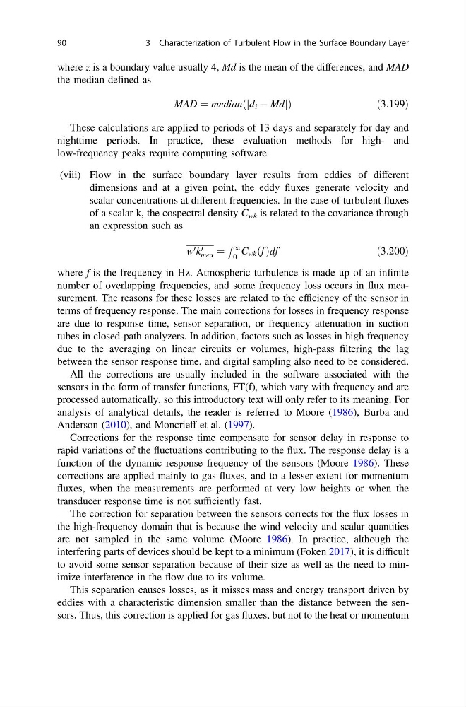
where z is a boundary value usually 4, Md is the mean of the differences, and MAD
the median defined as
MAD ¼ median d i À Md
j
j
ð
Þ
ð3:199Þ
These calculations are applied to periods of 13 days and separately for day and
nighttime periods. In practice, these evaluation methods for high- and
low-frequency peaks require computing software.
(viii) Flow in the surface boundary layer results from eddies of different
dimensions and at a given point, the eddy fluxes generate velocity and
scalar concentrations at different frequencies. In the case of turbulent fluxes
of a scalar k, the cospectral density C wk is related to the covariance through
an expression such as
w 0 k 0
mea ¼
Z 1
0
C wk ðf Þdf
ð3:200Þ
where f is the frequency in Hz. Atmospheric turbulence is made up of an infinite
number of overlapping frequencies, and some frequency loss occurs in flux measurement. The reasons for these losses are related to the efficiency of the sensor in
terms of frequency response. The main corrections for losses in frequency response
are due to response time, sensor separation, or frequency attenuation in suction
tubes in closed-path analyzers. In addition, factors such as losses in high frequency
due to the averaging on linear circuits or volumes, high-pass filtering the lag
between the sensor response time, and digital sampling also need to be considered.
All the corrections are usually included in the software associated with the
sensors in the form of transfer functions, FT(f), which vary with frequency and are
processed automatically, so this introductory text will only refer to its meaning. For
analysis of analytical details, the reader is referred to Moore (1986), Burba and
Anderson (2010), and Moncrieff et al. (1997).
Corrections for the response time compensate for sensor delay in response to
rapid variations of the fluctuations contributing to the flux. The response delay is a
function of the dynamic response frequency of the sensors (Moore 1986). These
corrections are applied mainly to gas fluxes, and to a lesser extent for momentum
fluxes, when the measurements are performed at very low heights or when the
transducer response time is not sufficiently fast.
The correction for separation between the sensors corrects for the flux losses in
the high-frequency domain that is because the wind velocity and scalar quantities
are not sampled in the same volume (Moore 1986). In practice, although the
interfering parts of devices should be kept to a minimum (Foken 2017), it is difficult
to avoid some sensor separation because of their size as well as the need to minimize interference in the flow due to its volume.
This separation causes losses, as it misses mass and energy transport driven by
eddies with a characteristic dimension smaller than the distance between the sensors. Thus, this correction is applied for gas fluxes, but not to the heat or momentum
90
3 Characterization of Turbulent Flow in the Surface Boundary Layer
the median defined as
MAD ¼ median d i À Md
j
j
ð
Þ
ð3:199Þ
These calculations are applied to periods of 13 days and separately for day and
nighttime periods. In practice, these evaluation methods for high- and
low-frequency peaks require computing software.
(viii) Flow in the surface boundary layer results from eddies of different
dimensions and at a given point, the eddy fluxes generate velocity and
scalar concentrations at different frequencies. In the case of turbulent fluxes
of a scalar k, the cospectral density C wk is related to the covariance through
an expression such as
w 0 k 0
mea ¼
Z 1
0
C wk ðf Þdf
ð3:200Þ
where f is the frequency in Hz. Atmospheric turbulence is made up of an infinite
number of overlapping frequencies, and some frequency loss occurs in flux measurement. The reasons for these losses are related to the efficiency of the sensor in
terms of frequency response. The main corrections for losses in frequency response
are due to response time, sensor separation, or frequency attenuation in suction
tubes in closed-path analyzers. In addition, factors such as losses in high frequency
due to the averaging on linear circuits or volumes, high-pass filtering the lag
between the sensor response time, and digital sampling also need to be considered.
All the corrections are usually included in the software associated with the
sensors in the form of transfer functions, FT(f), which vary with frequency and are
processed automatically, so this introductory text will only refer to its meaning. For
analysis of analytical details, the reader is referred to Moore (1986), Burba and
Anderson (2010), and Moncrieff et al. (1997).
Corrections for the response time compensate for sensor delay in response to
rapid variations of the fluctuations contributing to the flux. The response delay is a
function of the dynamic response frequency of the sensors (Moore 1986). These
corrections are applied mainly to gas fluxes, and to a lesser extent for momentum
fluxes, when the measurements are performed at very low heights or when the
transducer response time is not sufficiently fast.
The correction for separation between the sensors corrects for the flux losses in
the high-frequency domain that is because the wind velocity and scalar quantities
are not sampled in the same volume (Moore 1986). In practice, although the
interfering parts of devices should be kept to a minimum (Foken 2017), it is difficult
to avoid some sensor separation because of their size as well as the need to minimize interference in the flow due to its volume.
This separation causes losses, as it misses mass and energy transport driven by
eddies with a characteristic dimension smaller than the distance between the sensors. Thus, this correction is applied for gas fluxes, but not to the heat or momentum
90
3 Characterization of Turbulent Flow in the Surface Boundary Layer