

PyHasse, a Software Package for Applicational Studies of Partial Orderings
301
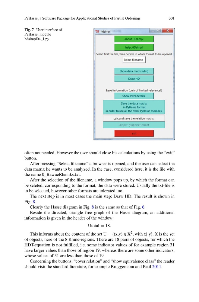
Fig. 7 User interface of
PyHasse, module
hdsimpl04_1.py
often not needed. However the user should close his calculations by using the “exit”
button.
After pressing “Select filename” a browser is opened, and the user can select the
data matrix he wants to be analyzed. In the case, considered here, it is the file with
the name 0_BawueRheinks.txt.
After the selection of the filename, a window pops up, by which the format can
be seleted, corresponding to the format, the data were stored. Usually the txt-file is
to be selected, however other formats are tolerated too.
The next step is in most cases the main step: Draw HD. The result is shown in
Fig. 8.
Clearly the Hasse diagram in Fig. 8 is the same as that of Fig. 6.
Beside the directed, triangle free graph of the Hasse diagram, an additional
information is given in the header of the window:
Utotal = 18.
This informs about the content of the set U = {(x,y) ∈ X 2 , with x||y}. X is the set
of objects, here of the 8 Rhine-regions. There are 18 pairs of objects, for which the
HDT-equation is not fulfilled, i.e. some indicator values of for example region 31
have larger values than those of region 19, whereas there are some other indicators,
whose values of 31 are less than those of 19.
Concerning the buttons, “cover relation” and “show equivalence class” the reader
should visit the standard literature, for example Bruggemann and Patil 2011.
301
Fig. 7 User interface of
PyHasse, module
hdsimpl04_1.py
often not needed. However the user should close his calculations by using the “exit”
button.
After pressing “Select filename” a browser is opened, and the user can select the
data matrix he wants to be analyzed. In the case, considered here, it is the file with
the name 0_BawueRheinks.txt.
After the selection of the filename, a window pops up, by which the format can
be seleted, corresponding to the format, the data were stored. Usually the txt-file is
to be selected, however other formats are tolerated too.
The next step is in most cases the main step: Draw HD. The result is shown in
Fig. 8.
Clearly the Hasse diagram in Fig. 8 is the same as that of Fig. 6.
Beside the directed, triangle free graph of the Hasse diagram, an additional
information is given in the header of the window:
Utotal = 18.
This informs about the content of the set U = {(x,y) ∈ X 2 , with x||y}. X is the set
of objects, here of the 8 Rhine-regions. There are 18 pairs of objects, for which the
HDT-equation is not fulfilled, i.e. some indicator values of for example region 31
have larger values than those of region 19, whereas there are some other indicators,
whose values of 31 are less than those of 19.
Concerning the buttons, “cover relation” and “show equivalence class” the reader
should visit the standard literature, for example Bruggemann and Patil 2011.