

412
7.3. EULER’S METHOD
0.4
0.8
1.2
0.4
0.8
1.2
t
y
0.4
0.8
1.2
0.4
0.8
1.2
t
y
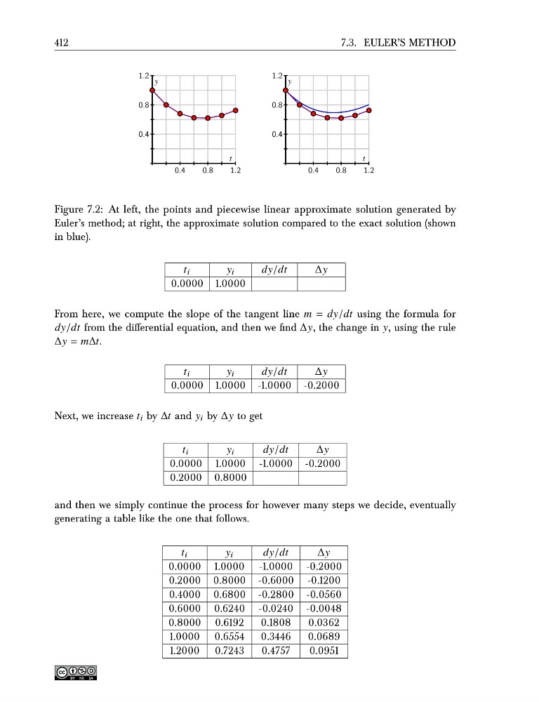
Figure 7.2: At left, the points and piecewise linear approximate solution generated by
Euler’s method; at right, the approximate solution compared to the exact solution (shown
in blue).
t i
y i
dy/dt
∆y
0.0000 1.0000
From here, we compute the slope of the tangent line m = dy/dt using the formula for
dy/dt from the differential equation, and then we find ∆y, the change in y, using the rule
∆y = m∆t.
t i
y i
dy/dt
∆y
0.0000 1.0000 -1.0000 -0.2000
Next, we increase t i by ∆t and y i by ∆y to get
t i
y i
dy/dt
∆y
0.0000 1.0000 -1.0000 -0.2000
0.2000 0.8000
and then we simply continue the process for however many steps we decide, eventually
generating a table like the one that follows.
t i
y i
dy/dt
∆y
0.0000 1.0000 -1.0000 -0.2000
0.2000 0.8000 -0.6000 -0.1200
0.4000 0.6800 -0.2800 -0.0560
0.6000 0.6240 -0.0240 -0.0048
0.8000 0.6192
0.1808
0.0362
1.0000 0.6554 0.3446
0.0689
1.2000 0.7243
0.4757
0.0951
7.3. EULER’S METHOD
0.4
0.8
1.2
0.4
0.8
1.2
t
y
0.4
0.8
1.2
0.4
0.8
1.2
t
y
Figure 7.2: At left, the points and piecewise linear approximate solution generated by
Euler’s method; at right, the approximate solution compared to the exact solution (shown
in blue).
t i
y i
dy/dt
∆y
0.0000 1.0000
From here, we compute the slope of the tangent line m = dy/dt using the formula for
dy/dt from the differential equation, and then we find ∆y, the change in y, using the rule
∆y = m∆t.
t i
y i
dy/dt
∆y
0.0000 1.0000 -1.0000 -0.2000
Next, we increase t i by ∆t and y i by ∆y to get
t i
y i
dy/dt
∆y
0.0000 1.0000 -1.0000 -0.2000
0.2000 0.8000
and then we simply continue the process for however many steps we decide, eventually
generating a table like the one that follows.
t i
y i
dy/dt
∆y
0.0000 1.0000 -1.0000 -0.2000
0.2000 0.8000 -0.6000 -0.1200
0.4000 0.6800 -0.2800 -0.0560
0.6000 0.6240 -0.0240 -0.0048
0.8000 0.6192
0.1808
0.0362
1.0000 0.6554 0.3446
0.0689
1.2000 0.7243
0.4757
0.0951