

7.3. EULER’S METHOD
411
While there is an algorithm by which we can find an algebraic formula for the solution to
this initial value problem, and we can check that this solution is y(t) = t − 1 + 2e −t , we are
instead interested in generating an approximate solution by creating a sequence of points
(t i , y i ), where y i ≈ y(t i ). For this first example, we choose ∆t = 0.2.
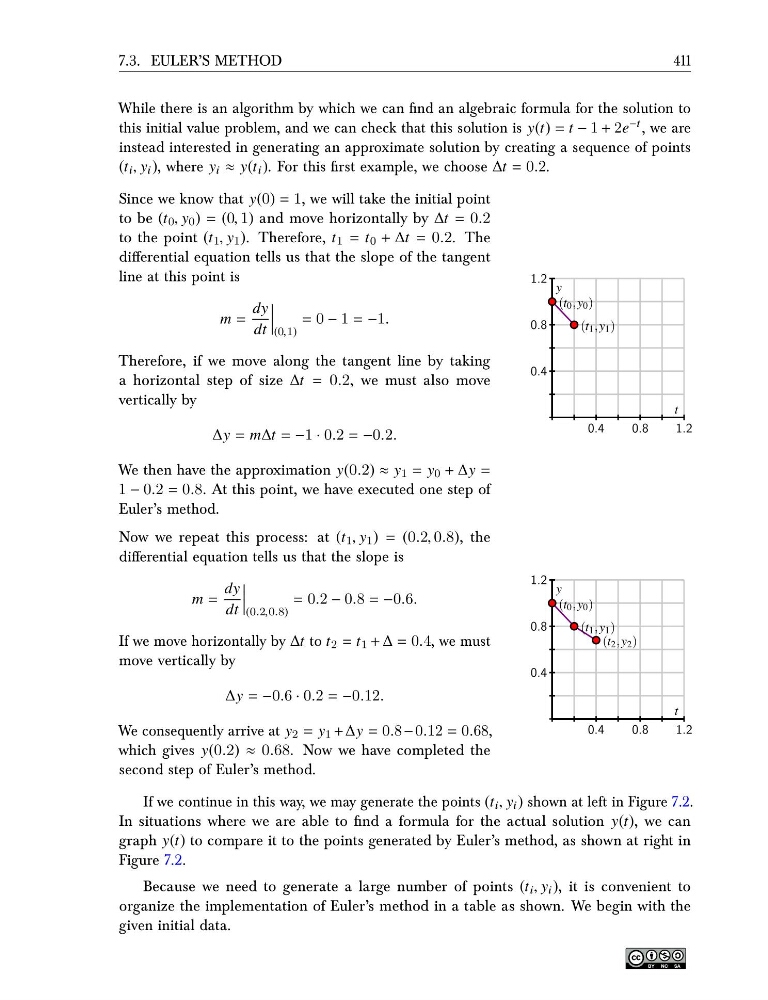
Since we know that y(0) = 1, we will take the initial point
to be (t 0 , y 0 ) = (0, 1) and move horizontally by ∆t = 0.2
to the point (t 1 , y 1 ). Therefore, t 1 = t 0 + ∆t = 0.2. The
differential equation tells us that the slope of the tangent
line at this point is
m =
dy
dt
(0,1)
= 0 − 1 = −1.
Therefore, if we move along the tangent line by taking
a horizontal step of size ∆t = 0.2, we must also move
vertically by
∆y = m∆t = −1 · 0.2 = −0.2.
We then have the approximation y(0.2) ≈ y 1 = y 0 + ∆y =
1 − 0.2 = 0.8. At this point, we have executed one step of
Euler’s method.
0.4
0.8
1.2
0.4
0.8
1.2
(t 0 , y 0 )
(t 1 , y 1 )
t
y
Now we repeat this process: at (t 1 , y 1 ) = (0.2, 0.8), the
differential equation tells us that the slope is
m =
dy
dt
(0.2,0.8)
= 0.2 − 0.8 = −0.6.
If we move horizontally by ∆t to t 2 = t 1 + ∆ = 0.4, we must
move vertically by
∆y = −0.6 · 0.2 = −0.12.
We consequently arrive at y 2 = y 1 + ∆y = 0.8 − 0.12 = 0.68,
which gives y(0.2) ≈ 0.68. Now we have completed the
second step of Euler’s method.
0.4
0.8
1.2
0.4
0.8
1.2
(t 0 , y 0 )
(t 1 , y 1 )
(t 2 , y 2 )
t
y
If we continue in this way, we may generate the points (t i , y i ) shown at left in Figure 7.2.
In situations where we are able to find a formula for the actual solution y(t), we can
graph y(t) to compare it to the points generated by Euler’s method, as shown at right in
Figure 7.2.
Because we need to generate a large number of points (t i , y i ), it is convenient to
organize the implementation of Euler’s method in a table as shown. We begin with the
given initial data.
411
While there is an algorithm by which we can find an algebraic formula for the solution to
this initial value problem, and we can check that this solution is y(t) = t − 1 + 2e −t , we are
instead interested in generating an approximate solution by creating a sequence of points
(t i , y i ), where y i ≈ y(t i ). For this first example, we choose ∆t = 0.2.
Since we know that y(0) = 1, we will take the initial point
to be (t 0 , y 0 ) = (0, 1) and move horizontally by ∆t = 0.2
to the point (t 1 , y 1 ). Therefore, t 1 = t 0 + ∆t = 0.2. The
differential equation tells us that the slope of the tangent
line at this point is
m =
dy
dt
(0,1)
= 0 − 1 = −1.
Therefore, if we move along the tangent line by taking
a horizontal step of size ∆t = 0.2, we must also move
vertically by
∆y = m∆t = −1 · 0.2 = −0.2.
We then have the approximation y(0.2) ≈ y 1 = y 0 + ∆y =
1 − 0.2 = 0.8. At this point, we have executed one step of
Euler’s method.
0.4
0.8
1.2
0.4
0.8
1.2
(t 0 , y 0 )
(t 1 , y 1 )
t
y
Now we repeat this process: at (t 1 , y 1 ) = (0.2, 0.8), the
differential equation tells us that the slope is
m =
dy
dt
(0.2,0.8)
= 0.2 − 0.8 = −0.6.
If we move horizontally by ∆t to t 2 = t 1 + ∆ = 0.4, we must
move vertically by
∆y = −0.6 · 0.2 = −0.12.
We consequently arrive at y 2 = y 1 + ∆y = 0.8 − 0.12 = 0.68,
which gives y(0.2) ≈ 0.68. Now we have completed the
second step of Euler’s method.
0.4
0.8
1.2
0.4
0.8
1.2
(t 0 , y 0 )
(t 1 , y 1 )
(t 2 , y 2 )
t
y
If we continue in this way, we may generate the points (t i , y i ) shown at left in Figure 7.2.
In situations where we are able to find a formula for the actual solution y(t), we can
graph y(t) to compare it to the points generated by Euler’s method, as shown at right in
Figure 7.2.
Because we need to generate a large number of points (t i , y i ), it is convenient to
organize the implementation of Euler’s method in a table as shown. We begin with the
given initial data.