

410
7.3. EULER’S METHOD
(c) Assuming that your approximation for y(2) is the actual value of y(2), use the
differential equation to find the slope of the tangent line to y(t) at t = 2. Then,
write the equation of the tangent line at t = 2.
(d) Add a sketch of this tangent line to your plot on the axes above on the interval
2 ≤ t ≤ 4; use this new tangent line to approximate y(4), the value of the solution
at t = 4.
(e) Repeat the same step to find an approximation for y(6).
⊲⊳
Euler’s Method
Preview Activity 7.3 demonstrates the essence of an algorithm, which is known as Euler’s
Method, that generates a numerical approximation to the solution of an initial value
problem. 3 In this algorithm, we will approximate the solution by taking horizontal steps of
a fixed size that we denote by ∆t.
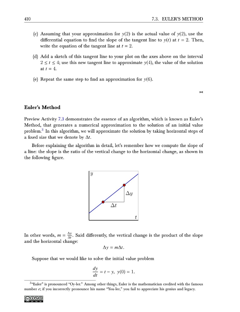
Before explaining the algorithm in detail, let’s remember how we compute the slope of
a line: the slope is the ratio of the vertical change to the horizontal change, as shown in
the following figure.
t
y
∆t
∆y
In other words, m =
∆y
∆t . Said differently, the vertical change is the product of the slope
and the horizontal change:
∆y = m∆t.
Suppose that we would like to solve the initial value problem
dy
dt
= t − y, y(0) = 1.
3 “Euler” is pronounced “Oy-ler.” Among other things, Euler is the mathematician credited with the famous
number e; if you incorrectly pronounce his name “You-ler,” you fail to appreciate his genius and legacy.
7.3. EULER’S METHOD
(c) Assuming that your approximation for y(2) is the actual value of y(2), use the
differential equation to find the slope of the tangent line to y(t) at t = 2. Then,
write the equation of the tangent line at t = 2.
(d) Add a sketch of this tangent line to your plot on the axes above on the interval
2 ≤ t ≤ 4; use this new tangent line to approximate y(4), the value of the solution
at t = 4.
(e) Repeat the same step to find an approximation for y(6).
⊲⊳
Euler’s Method
Preview Activity 7.3 demonstrates the essence of an algorithm, which is known as Euler’s
Method, that generates a numerical approximation to the solution of an initial value
problem. 3 In this algorithm, we will approximate the solution by taking horizontal steps of
a fixed size that we denote by ∆t.
Before explaining the algorithm in detail, let’s remember how we compute the slope of
a line: the slope is the ratio of the vertical change to the horizontal change, as shown in
the following figure.
t
y
∆t
∆y
In other words, m =
∆y
∆t . Said differently, the vertical change is the product of the slope
and the horizontal change:
∆y = m∆t.
Suppose that we would like to solve the initial value problem
dy
dt
= t − y, y(0) = 1.
3 “Euler” is pronounced “Oy-ler.” Among other things, Euler is the mathematician credited with the famous
number e; if you incorrectly pronounce his name “You-ler,” you fail to appreciate his genius and legacy.