

7.3. EULER’S METHOD
413
Activity 7.6.
Consider the initial value problem
dy
dt
= 2t − 1, y(0) = 0
(a) Use Euler’s method with ∆t = 0.2 to approximate the solution at t i =
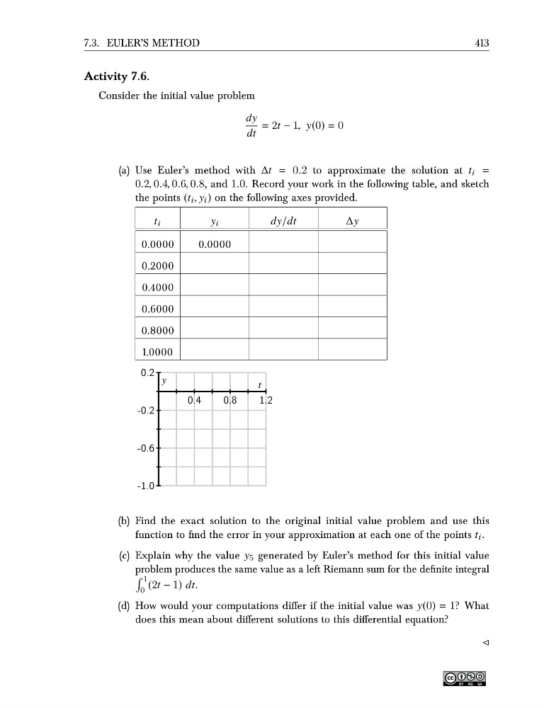
0.2, 0.4, 0.6, 0.8, and 1.0. Record your work in the following table, and sketch
the points (t i , y i ) on the following axes provided.
t i
y i
dy/dt
∆y
0.0000
0.0000
0.2000
0.4000
0.6000
0.8000
1.0000
0.4
0.8
1.2
-1.0
-0.6
-0.2
0.2
t
y
(b) Find the exact solution to the original initial value problem and use this
function to find the error in your approximation at each one of the points t i .
(c) Explain why the value y 5 generated by Euler’s method for this initial value
problem produces the same value as a left Riemann sum for the definite integral
1
0
(2t − 1) dt.
(d) How would your computations differ if the initial value was y(0) = 1? What
does this mean about different solutions to this differential equation?
⊳
413
Activity 7.6.
Consider the initial value problem
dy
dt
= 2t − 1, y(0) = 0
(a) Use Euler’s method with ∆t = 0.2 to approximate the solution at t i =
0.2, 0.4, 0.6, 0.8, and 1.0. Record your work in the following table, and sketch
the points (t i , y i ) on the following axes provided.
t i
y i
dy/dt
∆y
0.0000
0.0000
0.2000
0.4000
0.6000
0.8000
1.0000
0.4
0.8
1.2
-1.0
-0.6
-0.2
0.2
t
y
(b) Find the exact solution to the original initial value problem and use this
function to find the error in your approximation at each one of the points t i .
(c) Explain why the value y 5 generated by Euler’s method for this initial value
problem produces the same value as a left Riemann sum for the definite integral
1
0
(2t − 1) dt.
(d) How would your computations differ if the initial value was y(0) = 1? What
does this mean about different solutions to this differential equation?
⊳