

3.2. USING DERIVATIVES TO DESCRIBE FAMILIES OF FUNCTIONS
177
Note particularly that in g ′ (x) = ae −bx (1 − bx), the term ae −bx is always positive, so
the sign depends on the linear term (1 − bx), which is zero when x =
1
b . Note that this line
has negative slope (−b), so (1 − bx) is positive for x <
1
b and negative for x >
1
b . Hence
we can not only conclude that g is always increasing for x <
1
b and decreasing for x >
1
b ,
but also that g has a global maximum at (
1
b , g(
1
b )) and no local minimum.
We turn next to analyzing the concavity of g. With g ′ (x) = −abxe −bx + ae −bx , we
differentiate to find that
g
′′ (x) = −abxe
−bx (−b) + e
−bx (−ab) + ae
−bx (−b).
Combining like terms and factoring, we now have
g
′′ (x) = ab
2 xe
−bx − 2abe
−bx = abe
−bx (bx − 2).
Similar to our work with the first derivative, we observe that abe −bx is always positive,
sign(g ′′ )
behav(g)
+−
−
CCD
2
b
++
+
CCU
g ′′ (x) = abe −bx (bx − 2)
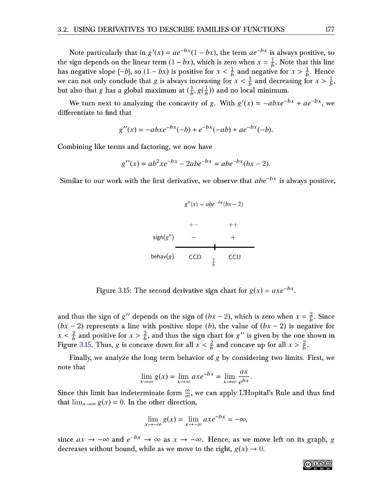
Figure 3.15: The second derivative sign chart for g(x) = axe −bx .
and thus the sign of g ′′ depends on the sign of (bx − 2), which is zero when x =
2
b . Since
(bx − 2) represents a line with positive slope (b), the value of (bx − 2) is negative for
x <
2
b and positive for x >
2
b , and thus the sign chart for g ′′ is given by the one shown in
Figure 3.15. Thus, g is concave down for all x <
2
b and concave up for all x >
2
b .
Finally, we analyze the long term behavior of g by considering two limits. First, we
note that
lim
x→∞
g(x) = lim
x→∞
axe
−bx = lim
x→∞
ax
e bx .
Since this limit has indeterminate form
∞
∞ , we can apply L’Hopital’s Rule and thus find
that lim x→∞ g(x) = 0. In the other direction,
lim
x→−∞
g(x) = lim
x→−∞
axe
−bx = −∞,
since ax → −∞ and e −bx → ∞ as x → −∞. Hence, as we move left on its graph, g
decreases without bound, while as we move to the right, g(x) → 0.
177
Note particularly that in g ′ (x) = ae −bx (1 − bx), the term ae −bx is always positive, so
the sign depends on the linear term (1 − bx), which is zero when x =
1
b . Note that this line
has negative slope (−b), so (1 − bx) is positive for x <
1
b and negative for x >
1
b . Hence
we can not only conclude that g is always increasing for x <
1
b and decreasing for x >
1
b ,
but also that g has a global maximum at (
1
b , g(
1
b )) and no local minimum.
We turn next to analyzing the concavity of g. With g ′ (x) = −abxe −bx + ae −bx , we
differentiate to find that
g
′′ (x) = −abxe
−bx (−b) + e
−bx (−ab) + ae
−bx (−b).
Combining like terms and factoring, we now have
g
′′ (x) = ab
2 xe
−bx − 2abe
−bx = abe
−bx (bx − 2).
Similar to our work with the first derivative, we observe that abe −bx is always positive,
sign(g ′′ )
behav(g)
+−
−
CCD
2
b
++
+
CCU
g ′′ (x) = abe −bx (bx − 2)
Figure 3.15: The second derivative sign chart for g(x) = axe −bx .
and thus the sign of g ′′ depends on the sign of (bx − 2), which is zero when x =
2
b . Since
(bx − 2) represents a line with positive slope (b), the value of (bx − 2) is negative for
x <
2
b and positive for x >
2
b , and thus the sign chart for g ′′ is given by the one shown in
Figure 3.15. Thus, g is concave down for all x <
2
b and concave up for all x >
2
b .
Finally, we analyze the long term behavior of g by considering two limits. First, we
note that
lim
x→∞
g(x) = lim
x→∞
axe
−bx = lim
x→∞
ax
e bx .
Since this limit has indeterminate form
∞
∞ , we can apply L’Hopital’s Rule and thus find
that lim x→∞ g(x) = 0. In the other direction,
lim
x→−∞
g(x) = lim
x→−∞
axe
−bx = −∞,
since ax → −∞ and e −bx → ∞ as x → −∞. Hence, as we move left on its graph, g
decreases without bound, while as we move to the right, g(x) → 0.