

176
3.2. USING DERIVATIVES TO DESCRIBE FAMILIES OF FUNCTIONS
parameters), we can often make broad conclusions about how each member of the family
will appear. The fundamental steps for this analysis are essentially identical to the work
we did in Section 3.1, as we demonstrate through the following example.
Example 3.3. Consider the two-parameter family of functions given by g(x) = axe −bx ,
where a and b are positive real numbers. Fully describe the behavior of a typical member
of the family in terms of a and b, including the location of all critical numbers, where g is
increasing, decreasing, concave up, and concave down, and the long term behavior of g.
Solution. We begin by computing g ′ (x). By the product rule,
g
′ (x) = ax
d
dx
e
−bx
+ e
−bx d
dx
[ax],
and thus by applying the chain rule and constant multiple rule, we find that
g
′ (x) = axe
−bx (−b) + e
−bx (a).
To find the critical numbers of g, we solve the equation g ′ (x) = 0. Here, it is especially
helpful to factor g ′ (x). We thus observe that setting the derivative equal to zero implies
0 = ae
−bx (−bx + 1).
Since we are given that a 0 and we know that e −bx 0 for all values of x, the only way
the preceding equation can hold is when −bx + 1 = 0. Solving for x, we find that x =
1
b ,
and this is therefore the only critical number of g.
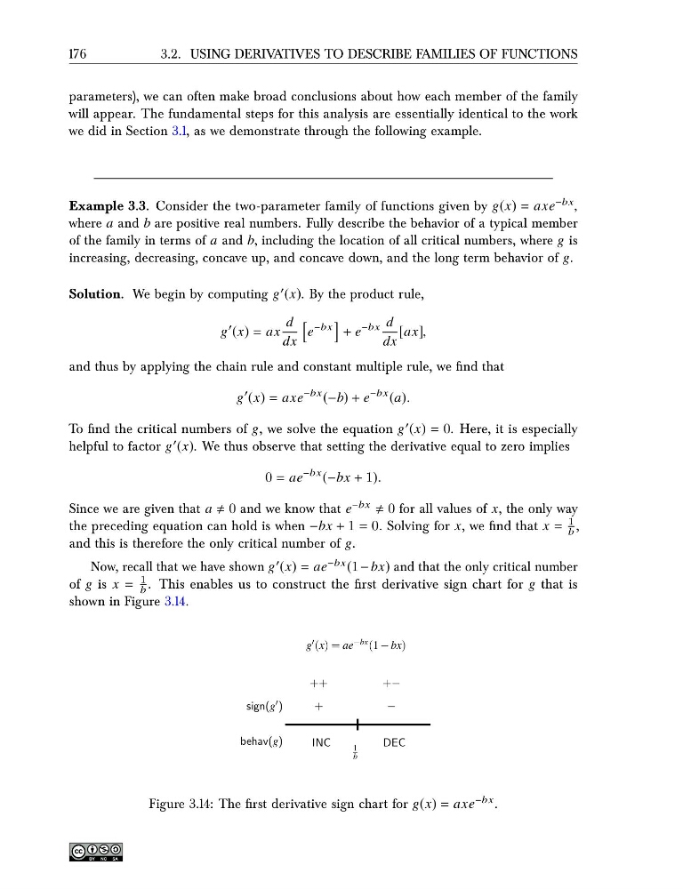
Now, recall that we have shown g ′ (x) = ae −bx (1 − bx) and that the only critical number
of g is x =
1
b . This enables us to construct the first derivative sign chart for g that is
shown in Figure 3.14.
sign(g ′ )
behav(g)
++
+
INC
1
b
+−
−
DEC
g ′ (x) = ae −bx (1 − bx)
Figure 3.14: The first derivative sign chart for g(x) = axe −bx .
3.2. USING DERIVATIVES TO DESCRIBE FAMILIES OF FUNCTIONS
parameters), we can often make broad conclusions about how each member of the family
will appear. The fundamental steps for this analysis are essentially identical to the work
we did in Section 3.1, as we demonstrate through the following example.
Example 3.3. Consider the two-parameter family of functions given by g(x) = axe −bx ,
where a and b are positive real numbers. Fully describe the behavior of a typical member
of the family in terms of a and b, including the location of all critical numbers, where g is
increasing, decreasing, concave up, and concave down, and the long term behavior of g.
Solution. We begin by computing g ′ (x). By the product rule,
g
′ (x) = ax
d
dx
e
−bx
+ e
−bx d
dx
[ax],
and thus by applying the chain rule and constant multiple rule, we find that
g
′ (x) = axe
−bx (−b) + e
−bx (a).
To find the critical numbers of g, we solve the equation g ′ (x) = 0. Here, it is especially
helpful to factor g ′ (x). We thus observe that setting the derivative equal to zero implies
0 = ae
−bx (−bx + 1).
Since we are given that a 0 and we know that e −bx 0 for all values of x, the only way
the preceding equation can hold is when −bx + 1 = 0. Solving for x, we find that x =
1
b ,
and this is therefore the only critical number of g.
Now, recall that we have shown g ′ (x) = ae −bx (1 − bx) and that the only critical number
of g is x =
1
b . This enables us to construct the first derivative sign chart for g that is
shown in Figure 3.14.
sign(g ′ )
behav(g)
++
+
INC
1
b
+−
−
DEC
g ′ (x) = ae −bx (1 − bx)
Figure 3.14: The first derivative sign chart for g(x) = axe −bx .