

178
3.2. USING DERIVATIVES TO DESCRIBE FAMILIES OF FUNCTIONS
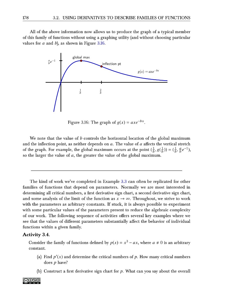
All of the above information now allows us to produce the graph of a typical member
of this family of functions without using a graphing utility (and without choosing particular
values for a and b), as shown in Figure 3.16.
1
b
global max
a
b e −1
2
b
inflection pt
g(x) = axe −bx
Figure 3.16: The graph of g(x) = axe −bx .
We note that the value of b controls the horizontal location of the global maximum
and the inflection point, as neither depends on a. The value of a affects the vertical stretch
of the graph. For example, the global maximum occurs at the point (
1
b , g(
1
b )) = (
1
b ,
a
b e −1 ),
so the larger the value of a, the greater the value of the global maximum.
The kind of work we’ve completed in Example 3.3 can often be replicated for other
families of functions that depend on parameters. Normally we are most interested in
determining all critical numbers, a first derivative sign chart, a second derivative sign chart,
and some analysis of the limit of the function as x → ∞. Throughout, we strive to work
with the parameters as arbitrary constants. If stuck, it is always possible to experiment
with some particular values of the parameters present to reduce the algebraic complexity
of our work. The following sequence of activities offers several key examples where we
see that the values of different parameters substantially affect the behavior of individual
functions within a given family.
Activity 3.4.
Consider the family of functions defined by p(x) = x 3 − ax, where a 0 is an arbitrary
constant.
(a) Find p ′ (x) and determine the critical numbers of p. How many critical numbers
does p have?
(b) Construct a first derivative sign chart for p. What can you say about the overall
3.2. USING DERIVATIVES TO DESCRIBE FAMILIES OF FUNCTIONS
All of the above information now allows us to produce the graph of a typical member
of this family of functions without using a graphing utility (and without choosing particular
values for a and b), as shown in Figure 3.16.
1
b
global max
a
b e −1
2
b
inflection pt
g(x) = axe −bx
Figure 3.16: The graph of g(x) = axe −bx .
We note that the value of b controls the horizontal location of the global maximum
and the inflection point, as neither depends on a. The value of a affects the vertical stretch
of the graph. For example, the global maximum occurs at the point (
1
b , g(
1
b )) = (
1
b ,
a
b e −1 ),
so the larger the value of a, the greater the value of the global maximum.
The kind of work we’ve completed in Example 3.3 can often be replicated for other
families of functions that depend on parameters. Normally we are most interested in
determining all critical numbers, a first derivative sign chart, a second derivative sign chart,
and some analysis of the limit of the function as x → ∞. Throughout, we strive to work
with the parameters as arbitrary constants. If stuck, it is always possible to experiment
with some particular values of the parameters present to reduce the algebraic complexity
of our work. The following sequence of activities offers several key examples where we
see that the values of different parameters substantially affect the behavior of individual
functions within a given family.
Activity 3.4.
Consider the family of functions defined by p(x) = x 3 − ax, where a 0 is an arbitrary
constant.
(a) Find p ′ (x) and determine the critical numbers of p. How many critical numbers
does p have?
(b) Construct a first derivative sign chart for p. What can you say about the overall