

3.1. USING DERIVATIVES TO IDENTIFY EXTREME VALUES
169
possible graph of f in Figure 3.8. The point A = (−
√
3, f (−
√
3)) is a local maximum, as
−
√
3 −
√
1.5
√
3
√
1.5
A
E
D
B
C
f
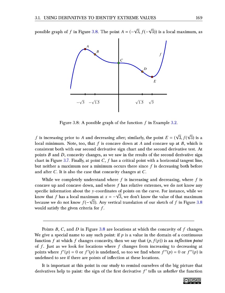
Figure 3.8: A possible graph of the function f in Example 3.2.
f is increasing prior to A and decreasing after; similarly, the point E = (
√
3, f (
√
3) is a
local minimum. Note, too, that f is concave down at A and concave up at B, which is
consistent both with our second derivative sign chart and the second derivative test. At
points B and D, concavity changes, as we saw in the results of the second derivative sign
chart in Figure 3.7. Finally, at point C, f has a critical point with a horizontal tangent line,
but neither a maximum nor a minimum occurs there since f is decreasing both before
and after C. It is also the case that concavity changes at C.
While we completely understand where f is increasing and decreasing, where f is
concave up and concave down, and where f has relative extremes, we do not know any
specific information about the y-coordinates of points on the curve. For instance, while we
know that f has a local maximum at x = −
√
3, we don’t know the value of that maximum
because we do not know f (−
√
3). Any vertical translation of our sketch of f in Figure 3.8
would satisfy the given criteria for f .
Points B, C, and D in Figure 3.8 are locations at which the concavity of f changes.
We give a special name to any such point: if p is a value in the domain of a continuous
function f at which f changes concavity, then we say that (p, f (p)) is an inflection point
of f . Just as we look for locations where f changes from increasing to decreasing at
points where f ′ (p) = 0 or f ′ (p) is undefined, so too we find where f ′′ (p) = 0 or f ′′ (p) is
undefined to see if there are points of inflection at these locations.
It is important at this point in our study to remind ourselves of the big picture that
derivatives help to paint: the sign of the first derivative f ′ tells us whether the function
169
possible graph of f in Figure 3.8. The point A = (−
√
3, f (−
√
3)) is a local maximum, as
−
√
3 −
√
1.5
√
3
√
1.5
A
E
D
B
C
f
Figure 3.8: A possible graph of the function f in Example 3.2.
f is increasing prior to A and decreasing after; similarly, the point E = (
√
3, f (
√
3) is a
local minimum. Note, too, that f is concave down at A and concave up at B, which is
consistent both with our second derivative sign chart and the second derivative test. At
points B and D, concavity changes, as we saw in the results of the second derivative sign
chart in Figure 3.7. Finally, at point C, f has a critical point with a horizontal tangent line,
but neither a maximum nor a minimum occurs there since f is decreasing both before
and after C. It is also the case that concavity changes at C.
While we completely understand where f is increasing and decreasing, where f is
concave up and concave down, and where f has relative extremes, we do not know any
specific information about the y-coordinates of points on the curve. For instance, while we
know that f has a local maximum at x = −
√
3, we don’t know the value of that maximum
because we do not know f (−
√
3). Any vertical translation of our sketch of f in Figure 3.8
would satisfy the given criteria for f .
Points B, C, and D in Figure 3.8 are locations at which the concavity of f changes.
We give a special name to any such point: if p is a value in the domain of a continuous
function f at which f changes concavity, then we say that (p, f (p)) is an inflection point
of f . Just as we look for locations where f changes from increasing to decreasing at
points where f ′ (p) = 0 or f ′ (p) is undefined, so too we find where f ′′ (p) = 0 or f ′′ (p) is
undefined to see if there are points of inflection at these locations.
It is important at this point in our study to remind ourselves of the big picture that
derivatives help to paint: the sign of the first derivative f ′ tells us whether the function