

168
3.1. USING DERIVATIVES TO IDENTIFY EXTREME VALUES
sign( f ′ )
behav( f )
+ − −
+
INC −
√
3
+ + −
−
DEC
0
+ + −
−
DEC
√
3
+ + +
+
INC
f ′ (x) = 3x 2 (x +
√
3)(x −
√
3)
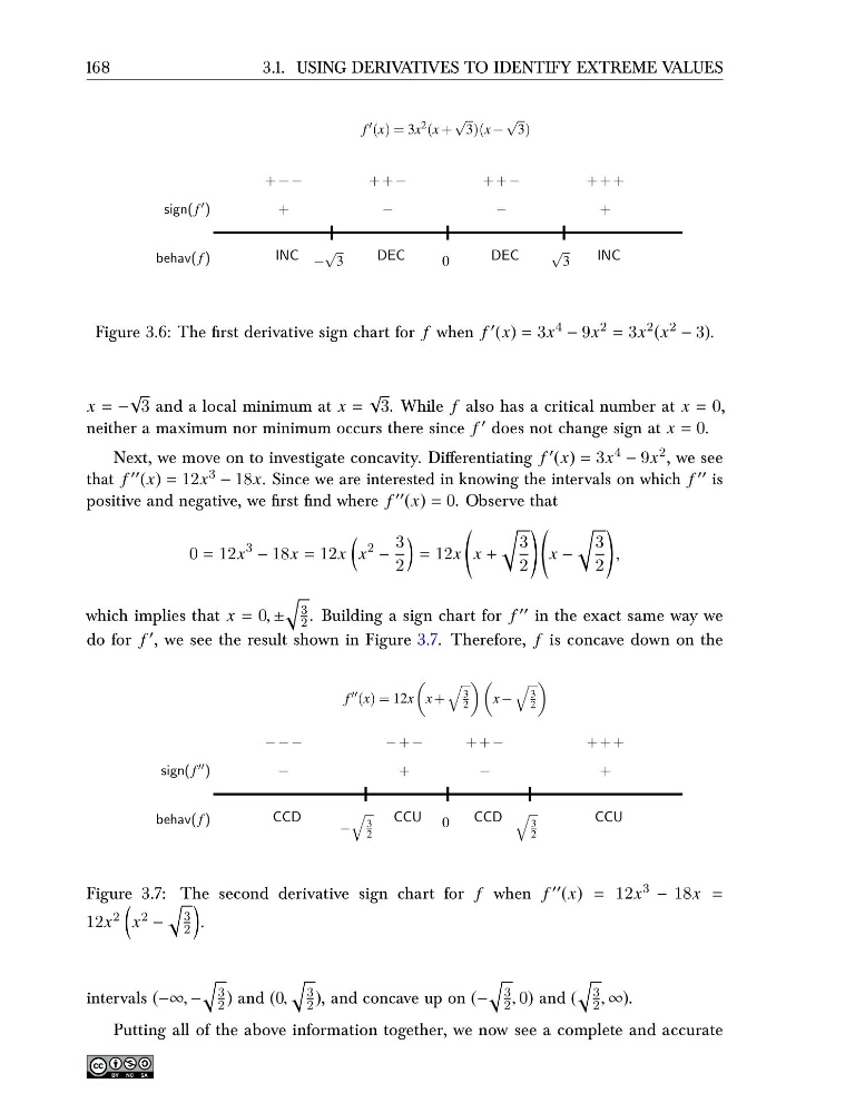
Figure 3.6: The first derivative sign chart for f when f ′ (x) = 3x 4 − 9x 2 = 3x 2 (x 2 − 3).
x = −
√
3 and a local minimum at x =
√
3. While f also has a critical number at x = 0,
neither a maximum nor minimum occurs there since f ′ does not change sign at x = 0.
Next, we move on to investigate concavity. Differentiating f ′ (x) = 3x 4 − 9x 2 , we see
that f ′′ (x) = 12x 3 − 18x. Since we are interested in knowing the intervals on which f ′′ is
positive and negative, we first find where f ′′ (x) = 0. Observe that
0 = 12x
3 − 18x = 12x
x
2 −
3
2
= 12x
x +
3
2
x −
3
2
,
which implies that x = 0, ±
3
2 . Building a sign chart for f ′′ in the exact same way we
do for f ′ , we see the result shown in Figure 3.7. Therefore, f is concave down on the
sign( f ′′ )
behav( f )
− − −
−
CCD
−
3
2
− + −
+
CCU 0
+ + −
−
CCD
3
2
+ + +
+
CCU
f ′′ (x) = 12x
x +
3
2
x −
3
2
Figure 3.7: The second derivative sign chart for f when f ′′ (x) = 12x 3 − 18x =
12x 2
x 2 −
3
2
.
intervals (−∞, −
3
2 ) and (0,
3
2 ), and concave up on (−
3
2 , 0) and (
3
2 , ∞).
Putting all of the above information together, we now see a complete and accurate
3.1. USING DERIVATIVES TO IDENTIFY EXTREME VALUES
sign( f ′ )
behav( f )
+ − −
+
INC −
√
3
+ + −
−
DEC
0
+ + −
−
DEC
√
3
+ + +
+
INC
f ′ (x) = 3x 2 (x +
√
3)(x −
√
3)
Figure 3.6: The first derivative sign chart for f when f ′ (x) = 3x 4 − 9x 2 = 3x 2 (x 2 − 3).
x = −
√
3 and a local minimum at x =
√
3. While f also has a critical number at x = 0,
neither a maximum nor minimum occurs there since f ′ does not change sign at x = 0.
Next, we move on to investigate concavity. Differentiating f ′ (x) = 3x 4 − 9x 2 , we see
that f ′′ (x) = 12x 3 − 18x. Since we are interested in knowing the intervals on which f ′′ is
positive and negative, we first find where f ′′ (x) = 0. Observe that
0 = 12x
3 − 18x = 12x
x
2 −
3
2
= 12x
x +
3
2
x −
3
2
,
which implies that x = 0, ±
3
2 . Building a sign chart for f ′′ in the exact same way we
do for f ′ , we see the result shown in Figure 3.7. Therefore, f is concave down on the
sign( f ′′ )
behav( f )
− − −
−
CCD
−
3
2
− + −
+
CCU 0
+ + −
−
CCD
3
2
+ + +
+
CCU
f ′′ (x) = 12x
x +
3
2
x −
3
2
Figure 3.7: The second derivative sign chart for f when f ′′ (x) = 12x 3 − 18x =
12x 2
x 2 −
3
2
.
intervals (−∞, −
3
2 ) and (0,
3
2 ), and concave up on (−
3
2 , 0) and (
3
2 , ∞).
Putting all of the above information together, we now see a complete and accurate