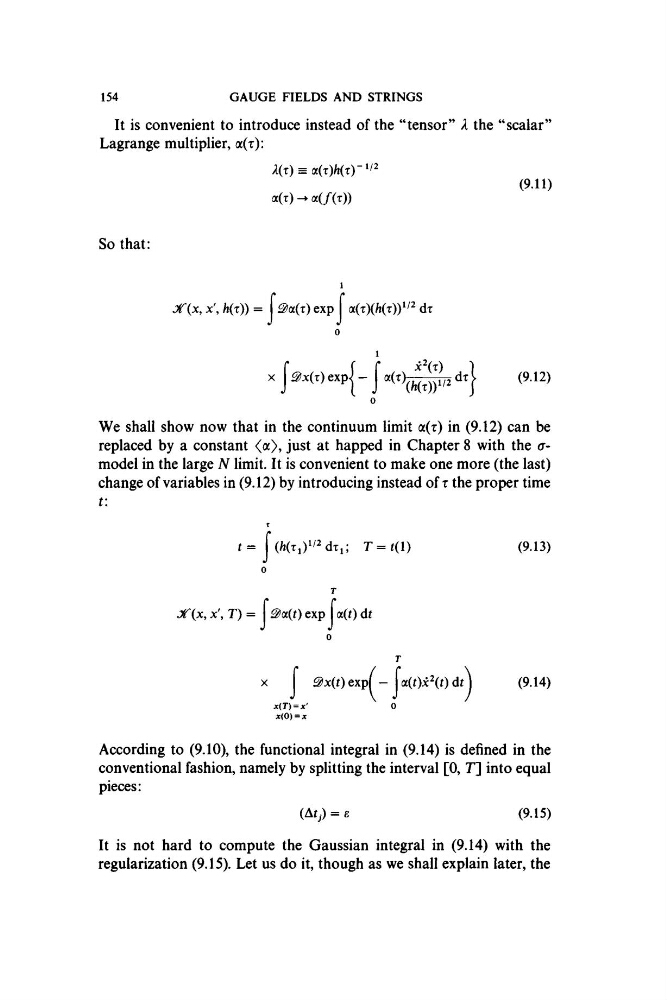
It is convenient to introduce instead of the “tensor” X the “scalar
Lagrange multiplier, a(r):
X{x) = a{x)h(x)-^i^
a(r) a(/(r))
154
GAUGE FIELDS AND STRINGS
(9.11)
So that:
jT(x, x ', h(x)) = 3>a{x) exp (x{T){h(T)y^^ dr
j® x (r) e x p j - I cc(x)~ ^^y,2 d tj
(9.12)
We shall show now that in the continuum limit a(r) in (9.12) can be
replaced by a constant , just at happed in Chapter 8 with the amodel in the large N limit. It is convenient to make one more (the last)
change of variables in (9.12) by introducing instead of t the proper time
t:
X
T = t(l)
(9.13)
j T ( x , x ', T) = S>(x{t) exp j*<^(0 di
0
^x(i)exp( -
x(T) = x'
x{0) = x
(x{t)x^(t) dt
(9.14)
According to (9.10), the functional integral in (9.14) is defined in the
conventional fashion, namely by splitting the interval [0, T] into equal
pieces:
(Ai,.) = £
(9.15)
It is not hard to compute the Gaussian integral in (9.14) with the
regularization (9.15). Let us do it, though as we shall explain later, the