

ANALOGIES BETWEEN GAUGE AND CHIRAL FIELDS
113
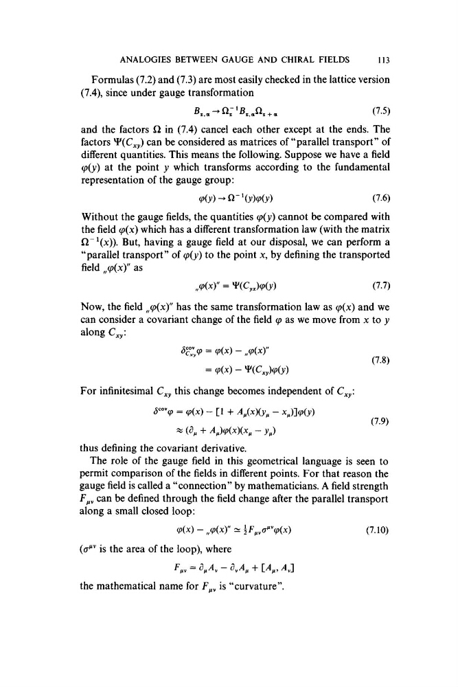
Formulas (7.2) and (7.3) are most easily checked in the lattice version
(7.4), since under gauge transformation
(7.5)
and the factors Q in (7.4) cancel each other except at the ends. The
factors ^(C^y) can be considered as matrices of “parallel transport” of
different quantities. This means the following. Suppose we have a field
(p{y) at the point y which transforms according to the fundamental
representation of the gauge group:
(p(y)-^n \y)(p{y)
(7.6)
Without the gauge fields, the quantities (p(y) cannot be compared with
the field cp(x) which has a different transformation law (with the matrix
Q"^(x)). But, having a gauge field at our disposal, we can perform a
“parallel transport” of (p(y) to the point x, by defining the transported
field „(p{x)" as
= ^(Cy^My)
(7.7)
Now, the field ^^cpix)" has the same transformation law as (p{x) and we
can consider a covariant change of the field cp as we move from x to y
along C^y i
s z y = cp(x) -
(7.8)
= cp{x) -
For infinitesimal C^y this change becomes independent of
= cp{x) - [1 + A^{x)(y^ - x ^ ) M y )
(7.9)
^ (^^ + ^^,)(p{x){x^ - y^)
thus defining the covariant derivative.
The role of the gauge field in this geometrical language is seen to
permit comparison of the fields in different points. For that reason the
gauge field is called a “connection” by mathematicians. A field strength
can be defined through the field change after the parallel transport
along a small closed loop:
- M ^y -
(cT^'’ is the area of the loop), where
the mathematical name for
is “curvature”.
(7.10)
113
Formulas (7.2) and (7.3) are most easily checked in the lattice version
(7.4), since under gauge transformation
(7.5)
and the factors Q in (7.4) cancel each other except at the ends. The
factors ^(C^y) can be considered as matrices of “parallel transport” of
different quantities. This means the following. Suppose we have a field
(p{y) at the point y which transforms according to the fundamental
representation of the gauge group:
(p(y)-^n \y)(p{y)
(7.6)
Without the gauge fields, the quantities (p(y) cannot be compared with
the field cp(x) which has a different transformation law (with the matrix
Q"^(x)). But, having a gauge field at our disposal, we can perform a
“parallel transport” of (p(y) to the point x, by defining the transported
field „(p{x)" as
= ^(Cy^My)
(7.7)
Now, the field ^^cpix)" has the same transformation law as (p{x) and we
can consider a covariant change of the field cp as we move from x to y
along C^y i
s z y = cp(x) -
(7.8)
= cp{x) -
For infinitesimal C^y this change becomes independent of
= cp{x) - [1 + A^{x)(y^ - x ^ ) M y )
(7.9)
^ (^^ + ^^,)(p{x){x^ - y^)
thus defining the covariant derivative.
The role of the gauge field in this geometrical language is seen to
permit comparison of the fields in different points. For that reason the
gauge field is called a “connection” by mathematicians. A field strength
can be defined through the field change after the parallel transport
along a small closed loop:
- M ^y -
(cT^'’ is the area of the loop), where
the mathematical name for
is “curvature”.
(7.10)