

568 Higher Engineering Mathematics
in Fig. 58.6. When plotting these values, it will always
be found that the co-ordinate for the 100% cumulative
frequency value cannot be plotted, since the maximum
value on the probability scale is 99.99. Since the points
plotted in Fig. 58.6 lie very nearly in a straight line,
the data is approximately normally distributed.
The mean value and standard deviation can be determined from Fig. 58.6. Since a normal curve is symmetrical, the mean value is the value of the variable
corresponding to a 50% cumulative frequency value,
shown as point P on the graph. This shows that the
mean value is 33.6 kg. The standard deviation is determined using the 84% and 16% cumulative frequency
values, shown as Q and R in Fig. 58.6. The variable values for Q and R are 35.7 and 31.4 respectively; thus two
standard deviations correspond to 35.7 − 31.4, i.e. 4.3,
showing that the standard deviation of the distribution
is approximately
4.3
2
i.e. 2.15 standard deviations.
The mean value and standard deviation of the distribution can be calculated using
mean, x =
f x
f
and standard deviation,
σ =
[ f (x − ¯
x )
2 ]
f
where f is the frequency of a class and x is the class midpoint value. Using these formulae gives a mean value
of the distribution of 33.6 (as obtained graphically) and
a standard deviation of 2.12, showing that the graphical
method of determining the mean and standard deviation
give quite realistic results.
Problem 6. Use normal probability paper to
determine whether the data given below is normally
distributed. Use the graph and assume a normal
distribution whether this is so or not, to find
approximate values of the mean and standard
deviation of the distribution.
Class mid-point values
Frequency
5
1
15
2
25
3
35
6
Class mid-point values
Frequency
45
9
55
6
65
2
75
2
85
1
95
1
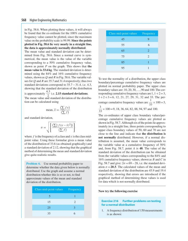
To test the normality of a distribution, the upper class
boundary/percentage cumulative frequency values are
plotted on normal probability paper. The upper class
boundary values are: 10, 20, 30, …, 90 and 100. The corresponding cumulative frequency values are 1, 1 +2 = 3,
1 + 2 +3 = 6, 12, 21, 27, 29, 31, 32 and 33. The percentage cumulative frequency values are
1
33
× 100 =3,
3
33
× 100 =9, 18, 36, 64, 82, 88, 94, 97 and 100.
The co-ordinates of upper class boundary values/percentage cumulative frequency values are plotted as
shown in Fig. 58.7. Although six of the points lie approximately in a straight line, three points corresponding to
upper class boundary values of 50, 60 and 70 are not
close to the line and indicate that the distribution is
not normally distributed. However, if a normal distribution is assumed, the mean value corresponds to
the variable value at a cumulative frequency of 50%
and, from Fig. 58.7, point A is 48. The value of the
standard deviation of the distribution can be obtained
from the variable values corresponding to the 84% and
16% cumulative frequency values, shown as B and C in
Fig. 58.7 and give: 2σ = 69 −28, i.e. the standard deviation σ = 20.5. The calculated values of the mean and
standard deviation of the distribution are 45.9 and 19.4
respectively, showing that errors are introduced if the
graphical method of determining these values is used
for data which is not normally distributed.
Now try the following exercise
Exercise 216 Further problems on testing
for a normal distribution
1. A frequency distribution of 150 measurements
is as shown:
in Fig. 58.6. When plotting these values, it will always
be found that the co-ordinate for the 100% cumulative
frequency value cannot be plotted, since the maximum
value on the probability scale is 99.99. Since the points
plotted in Fig. 58.6 lie very nearly in a straight line,
the data is approximately normally distributed.
The mean value and standard deviation can be determined from Fig. 58.6. Since a normal curve is symmetrical, the mean value is the value of the variable
corresponding to a 50% cumulative frequency value,
shown as point P on the graph. This shows that the
mean value is 33.6 kg. The standard deviation is determined using the 84% and 16% cumulative frequency
values, shown as Q and R in Fig. 58.6. The variable values for Q and R are 35.7 and 31.4 respectively; thus two
standard deviations correspond to 35.7 − 31.4, i.e. 4.3,
showing that the standard deviation of the distribution
is approximately
4.3
2
i.e. 2.15 standard deviations.
The mean value and standard deviation of the distribution can be calculated using
mean, x =
f x
f
and standard deviation,
σ =
[ f (x − ¯
x )
2 ]
f
where f is the frequency of a class and x is the class midpoint value. Using these formulae gives a mean value
of the distribution of 33.6 (as obtained graphically) and
a standard deviation of 2.12, showing that the graphical
method of determining the mean and standard deviation
give quite realistic results.
Problem 6. Use normal probability paper to
determine whether the data given below is normally
distributed. Use the graph and assume a normal
distribution whether this is so or not, to find
approximate values of the mean and standard
deviation of the distribution.
Class mid-point values
Frequency
5
1
15
2
25
3
35
6
Class mid-point values
Frequency
45
9
55
6
65
2
75
2
85
1
95
1
To test the normality of a distribution, the upper class
boundary/percentage cumulative frequency values are
plotted on normal probability paper. The upper class
boundary values are: 10, 20, 30, …, 90 and 100. The corresponding cumulative frequency values are 1, 1 +2 = 3,
1 + 2 +3 = 6, 12, 21, 27, 29, 31, 32 and 33. The percentage cumulative frequency values are
1
33
× 100 =3,
3
33
× 100 =9, 18, 36, 64, 82, 88, 94, 97 and 100.
The co-ordinates of upper class boundary values/percentage cumulative frequency values are plotted as
shown in Fig. 58.7. Although six of the points lie approximately in a straight line, three points corresponding to
upper class boundary values of 50, 60 and 70 are not
close to the line and indicate that the distribution is
not normally distributed. However, if a normal distribution is assumed, the mean value corresponds to
the variable value at a cumulative frequency of 50%
and, from Fig. 58.7, point A is 48. The value of the
standard deviation of the distribution can be obtained
from the variable values corresponding to the 84% and
16% cumulative frequency values, shown as B and C in
Fig. 58.7 and give: 2σ = 69 −28, i.e. the standard deviation σ = 20.5. The calculated values of the mean and
standard deviation of the distribution are 45.9 and 19.4
respectively, showing that errors are introduced if the
graphical method of determining these values is used
for data which is not normally distributed.
Now try the following exercise
Exercise 216 Further problems on testing
for a normal distribution
1. A frequency distribution of 150 measurements
is as shown: