

The normal distribution 567
30
32
34
36
38
40
42
0.01
0.05
0.1
0.2
0.5
1
2
5
10
20
30
40
50
60
70
80
90
95
98
99
99.8
99.9
99.99
Percentage cumulative frequency
Upper class boundary
Q
P
R
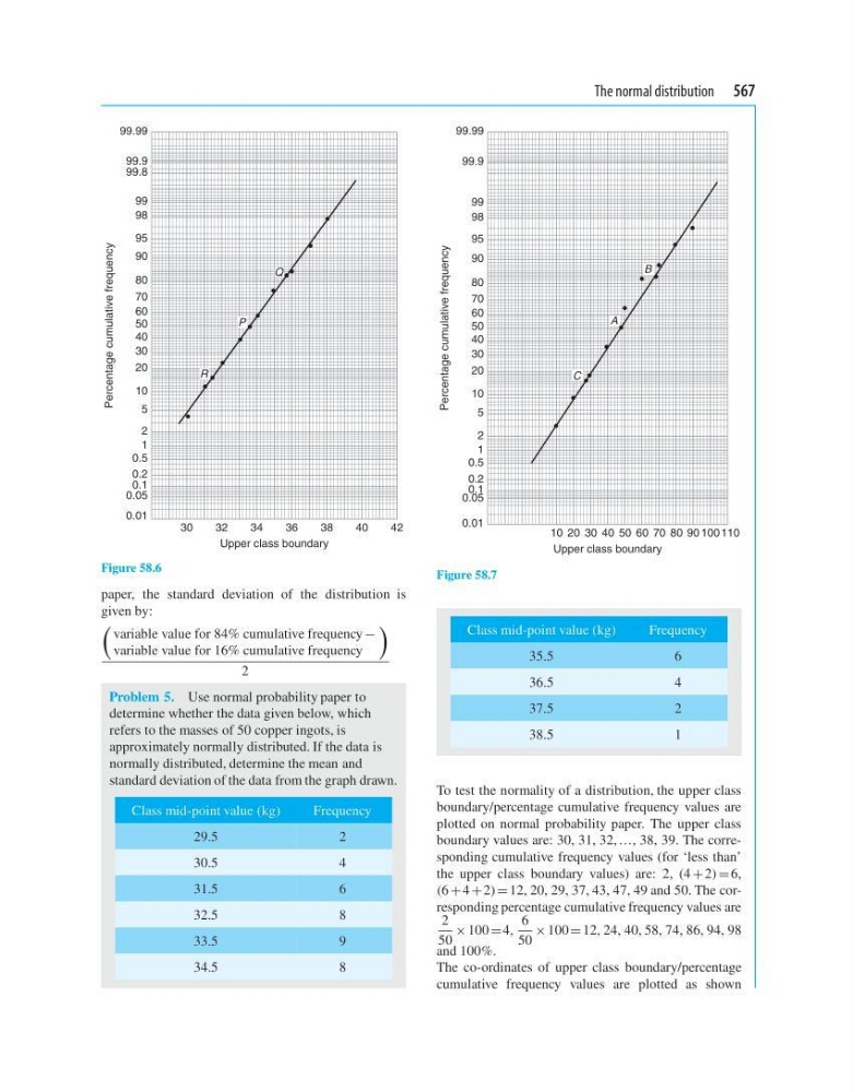
Figure 58.6
paper, the standard deviation of the distribution is
given by:
variable value for 84% cumulative frequency −
variable value for 16% cumulative frequency
2
Problem 5. Use normal probability paper to
determine whether the data given below, which
refers to the masses of 50 copper ingots, is
approximately normally distributed. If the data is
normally distributed, determine the mean and
standard deviation of the data from the graph drawn.
Class mid-point value (kg)
Frequency
29.5
2
30.5
4
31.5
6
32.5
8
33.5
9
34.5
8
0.01
0.05
0.1
0.2
0.5
1
2
5
10
20
30
40
50
60
70
80
90
95
98
99
99.9
99.99
Upper class boundary
Percentage cumulative frequency
B
A
C
10 20 30 40 50 60 70 80 90 100 110
Figure 58.7
Class mid-point value (kg)
Frequency
35.5
6
36.5
4
37.5
2
38.5
1
To test the normality of a distribution, the upper class
boundary/percentage cumulative frequency values are
plotted on normal probability paper. The upper class
boundary values are: 30, 31, 32, …, 38, 39. The corresponding cumulative frequency values (for ‘less than’
the upper class boundary values) are: 2, (4 + 2) = 6,
(6 + 4 +2) = 12, 20, 29, 37, 43, 47, 49 and 50. The corresponding percentage cumulative frequency values are
2
50
× 100 =4,
6
50
× 100 = 12, 24, 40, 58, 74, 86, 94, 98
and 100%.
The co-ordinates of upper class boundary/percentage
cumulative frequency values are plotted as shown
30
32
34
36
38
40
42
0.01
0.05
0.1
0.2
0.5
1
2
5
10
20
30
40
50
60
70
80
90
95
98
99
99.8
99.9
99.99
Percentage cumulative frequency
Upper class boundary
Q
P
R
Figure 58.6
paper, the standard deviation of the distribution is
given by:
variable value for 84% cumulative frequency −
variable value for 16% cumulative frequency
2
Problem 5. Use normal probability paper to
determine whether the data given below, which
refers to the masses of 50 copper ingots, is
approximately normally distributed. If the data is
normally distributed, determine the mean and
standard deviation of the data from the graph drawn.
Class mid-point value (kg)
Frequency
29.5
2
30.5
4
31.5
6
32.5
8
33.5
9
34.5
8
0.01
0.05
0.1
0.2
0.5
1
2
5
10
20
30
40
50
60
70
80
90
95
98
99
99.9
99.99
Upper class boundary
Percentage cumulative frequency
B
A
C
10 20 30 40 50 60 70 80 90 100 110
Figure 58.7
Class mid-point value (kg)
Frequency
35.5
6
36.5
4
37.5
2
38.5
1
To test the normality of a distribution, the upper class
boundary/percentage cumulative frequency values are
plotted on normal probability paper. The upper class
boundary values are: 30, 31, 32, …, 38, 39. The corresponding cumulative frequency values (for ‘less than’
the upper class boundary values) are: 2, (4 + 2) = 6,
(6 + 4 +2) = 12, 20, 29, 37, 43, 47, 49 and 50. The corresponding percentage cumulative frequency values are
2
50
× 100 =4,
6
50
× 100 = 12, 24, 40, 58, 74, 86, 94, 98
and 100%.
The co-ordinates of upper class boundary/percentage
cumulative frequency values are plotted as shown