

Chapter 58
The normal distribution
58.1 Introduction to the normal
distribution
When data is obtained, it can frequently be considered
to be a sample (i.e. a few members) drawn at random
from a large population (i.e. a set having many members). If the sample number is large, it is theoretically
possible to choose class intervals which are very small,
but which still have a number of members falling within
each class. A frequency polygon of this data then has a
large number of small line segments and approximates
to a continuous curve. Such a curve is called a frequency
or a distribution curve.
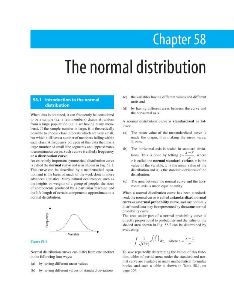
An extremely important symmetrical distribution curve
is called the normal curve and is as shown in Fig. 58.1.
This curve can be described by a mathematical equation and is the basis of much of the work done in more
advanced statistics. Many natural occurrences such as
the heights or weights of a group of people, the sizes
of components produced by a particular machine and
the life length of certain components approximate to a
normal distribution.
Variable
Frequency
Figure 58.1
Normal distribution curves can differ from one another
in the following four ways:
(a) by having different mean values
(b) by having different values of standard deviations
(c) the variables having different values and different
units and
(d) by having different areas between the curve and
the horizontal axis.
A normal distribution curve is standardized as follows:
(a) The mean value of the unstandardized curve is
made the origin, thus making the mean value,
x , zero.
(b) The horizontal axis is scaled in standard deviations. This is done by letting z =
x − x
σ
, where
z is called the normal standard variate, x is the
value of the variable, x is the mean value of the
distribution and σ is the standard deviation of the
distribution.
(c) The area between the normal curve and the horizontal axis is made equal to unity.
When a normal distribution curve has been standardized, the normal curve is called a standardized normal
curve or a normal probability curve, and any normally
distributed data may be represented by the same normal
probability curve.
The area under part of a normal probability curve is
directly proportional to probability and the value of the
shaded area shown in Fig. 58.2 can be determined by
evaluating:
1
√
(2π)
e
z 2
2
dz, where z =
x − x
σ
To save repeatedly determining the values of this function, tables of partial areas under the standardized normal curve are available in many mathematical formulae
books, and such a table is shown in Table 58.1, on
page 564.
The normal distribution
58.1 Introduction to the normal
distribution
When data is obtained, it can frequently be considered
to be a sample (i.e. a few members) drawn at random
from a large population (i.e. a set having many members). If the sample number is large, it is theoretically
possible to choose class intervals which are very small,
but which still have a number of members falling within
each class. A frequency polygon of this data then has a
large number of small line segments and approximates
to a continuous curve. Such a curve is called a frequency
or a distribution curve.
An extremely important symmetrical distribution curve
is called the normal curve and is as shown in Fig. 58.1.
This curve can be described by a mathematical equation and is the basis of much of the work done in more
advanced statistics. Many natural occurrences such as
the heights or weights of a group of people, the sizes
of components produced by a particular machine and
the life length of certain components approximate to a
normal distribution.
Variable
Frequency
Figure 58.1
Normal distribution curves can differ from one another
in the following four ways:
(a) by having different mean values
(b) by having different values of standard deviations
(c) the variables having different values and different
units and
(d) by having different areas between the curve and
the horizontal axis.
A normal distribution curve is standardized as follows:
(a) The mean value of the unstandardized curve is
made the origin, thus making the mean value,
x , zero.
(b) The horizontal axis is scaled in standard deviations. This is done by letting z =
x − x
σ
, where
z is called the normal standard variate, x is the
value of the variable, x is the mean value of the
distribution and σ is the standard deviation of the
distribution.
(c) The area between the normal curve and the horizontal axis is made equal to unity.
When a normal distribution curve has been standardized, the normal curve is called a standardized normal
curve or a normal probability curve, and any normally
distributed data may be represented by the same normal
probability curve.
The area under part of a normal probability curve is
directly proportional to probability and the value of the
shaded area shown in Fig. 58.2 can be determined by
evaluating:
1
√
(2π)
e
z 2
2
dz, where z =
x − x
σ
To save repeatedly determining the values of this function, tables of partial areas under the standardized normal curve are available in many mathematical formulae
books, and such a table is shown in Table 58.1, on
page 564.