

Presentation ofstatistical data 539
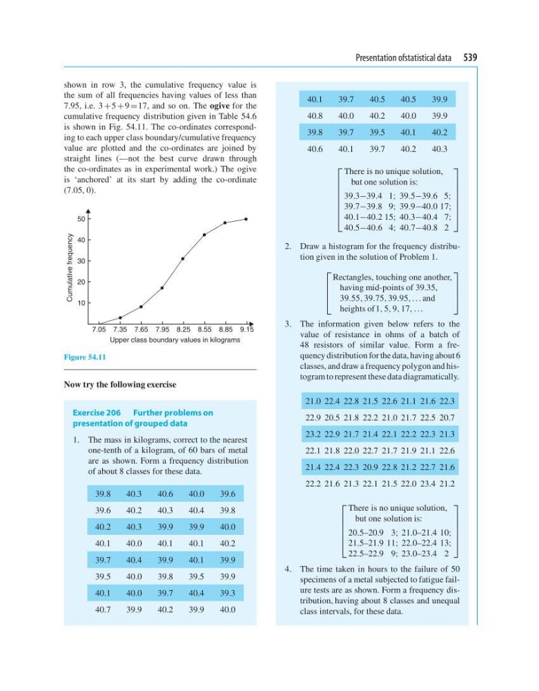
shown in row 3, the cumulative frequency value is
the sum of all frequencies having values of less than
7.95, i.e. 3 +5 + 9 =17, and so on. The ogive for the
cumulative frequency distribution given in Table 54.6
is shown in Fig. 54.11. The co-ordinates corresponding to each upper class boundary/cumulative frequency
value are plotted and the co-ordinates are joined by
straight lines (—not the best curve drawn through
the co-ordinates as in experimental work.) The ogive
is ‘anchored’ at its start by adding the co-ordinate
(7.05, 0).
7.05
10
Cumulative frequency
40
30
20
50
7.95
7.35 7.65
8.25
Upper class boundary values in kilograms
8.85 9.15
8.55
Figure 54.11
Now try the following exercise
Exercise 206 Further problems on
presentation of grouped data
1. The mass in kilograms, correct to the nearest
one-tenth of a kilogram, of 60 bars of metal
are as shown. Form a frequency distribution
of about 8 classes for these data.
39.8
40.3
40.6
40.0
39.6
39.6
40.2
40.3
40.4
39.8
40.2
40.3
39.9
39.9
40.0
40.1
40.0
40.1
40.1
40.2
39.7
40.4
39.9
40.1
39.9
39.5
40.0
39.8
39.5
39.9
40.1
40.0
39.7
40.4
39.3
40.7
39.9
40.2
39.9
40.0
40.1
39.7
40.5
40.5
39.9
40.8
40.0
40.2
40.0
39.9
39.8
39.7
39.5
40.1
40.2
40.6
40.1
39.7
40.2
40.3
⎡
⎢
⎢
⎢
⎢
⎢
⎢
⎣
There is no unique solution,
but one solution is:
39.3−39.4 1; 39.5−39.6 5;
39.7−39.8 9; 39.9−40.0 17;
40.1−40.2 15; 40.3−40.4 7;
40.5−40.6 4; 40.7−40.8 2
⎤
⎥
⎥
⎥
⎥
⎥
⎥
⎦
2. Draw a histogram for the frequency distribution given in the solution of Problem 1.
⎡
⎢
⎢
⎣
Rectangles, touching one another,
having mid-points of 39.35,
39.55, 39.75, 39.95,... and
heights of 1, 5, 9, 17, ...
⎤
⎥
⎥
⎦
3. The information given below refers to the
value of resistance in ohms of a batch of
48 resistors of similar value. Form a frequency distribution for the data, having about 6
classes, and draw a frequency polygon and histogram to represent these data diagramatically.
21.0 22.4 22.8 21.5 22.6 21.1 21.6 22.3
22.9 20.5 21.8 22.2 21.0 21.7 22.5 20.7
23.2 22.9 21.7 21.4 22.1 22.2 22.3 21.3
22.1 21.8 22.0 22.7 21.7 21.9 21.1 22.6
21.4 22.4 22.3 20.9 22.8 21.2 22.7 21.6
22.2 21.6 21.3 22.1 21.5 22.0 23.4 21.2
⎡
⎢
⎢
⎢
⎢
⎣
There is no unique solution,
but one solution is:
20.5–20.9 3; 21.0–21.4 10;
21.5–21.9 11; 22.0–22.4 13;
22.5–22.9 9; 23.0–23.4 2
⎤
⎥
⎥
⎥
⎥
⎦
4. The time taken in hours to the failure of 50
specimens of a metal subjected to fatigue failure tests are as shown. Form a frequency distribution, having about 8 classes and unequal
class intervals, for these data.
shown in row 3, the cumulative frequency value is
the sum of all frequencies having values of less than
7.95, i.e. 3 +5 + 9 =17, and so on. The ogive for the
cumulative frequency distribution given in Table 54.6
is shown in Fig. 54.11. The co-ordinates corresponding to each upper class boundary/cumulative frequency
value are plotted and the co-ordinates are joined by
straight lines (—not the best curve drawn through
the co-ordinates as in experimental work.) The ogive
is ‘anchored’ at its start by adding the co-ordinate
(7.05, 0).
7.05
10
Cumulative frequency
40
30
20
50
7.95
7.35 7.65
8.25
Upper class boundary values in kilograms
8.85 9.15
8.55
Figure 54.11
Now try the following exercise
Exercise 206 Further problems on
presentation of grouped data
1. The mass in kilograms, correct to the nearest
one-tenth of a kilogram, of 60 bars of metal
are as shown. Form a frequency distribution
of about 8 classes for these data.
39.8
40.3
40.6
40.0
39.6
39.6
40.2
40.3
40.4
39.8
40.2
40.3
39.9
39.9
40.0
40.1
40.0
40.1
40.1
40.2
39.7
40.4
39.9
40.1
39.9
39.5
40.0
39.8
39.5
39.9
40.1
40.0
39.7
40.4
39.3
40.7
39.9
40.2
39.9
40.0
40.1
39.7
40.5
40.5
39.9
40.8
40.0
40.2
40.0
39.9
39.8
39.7
39.5
40.1
40.2
40.6
40.1
39.7
40.2
40.3
⎡
⎢
⎢
⎢
⎢
⎢
⎢
⎣
There is no unique solution,
but one solution is:
39.3−39.4 1; 39.5−39.6 5;
39.7−39.8 9; 39.9−40.0 17;
40.1−40.2 15; 40.3−40.4 7;
40.5−40.6 4; 40.7−40.8 2
⎤
⎥
⎥
⎥
⎥
⎥
⎥
⎦
2. Draw a histogram for the frequency distribution given in the solution of Problem 1.
⎡
⎢
⎢
⎣
Rectangles, touching one another,
having mid-points of 39.35,
39.55, 39.75, 39.95,... and
heights of 1, 5, 9, 17, ...
⎤
⎥
⎥
⎦
3. The information given below refers to the
value of resistance in ohms of a batch of
48 resistors of similar value. Form a frequency distribution for the data, having about 6
classes, and draw a frequency polygon and histogram to represent these data diagramatically.
21.0 22.4 22.8 21.5 22.6 21.1 21.6 22.3
22.9 20.5 21.8 22.2 21.0 21.7 22.5 20.7
23.2 22.9 21.7 21.4 22.1 22.2 22.3 21.3
22.1 21.8 22.0 22.7 21.7 21.9 21.1 22.6
21.4 22.4 22.3 20.9 22.8 21.2 22.7 21.6
22.2 21.6 21.3 22.1 21.5 22.0 23.4 21.2
⎡
⎢
⎢
⎢
⎢
⎣
There is no unique solution,
but one solution is:
20.5–20.9 3; 21.0–21.4 10;
21.5–21.9 11; 22.0–22.4 13;
22.5–22.9 9; 23.0–23.4 2
⎤
⎥
⎥
⎥
⎥
⎦
4. The time taken in hours to the failure of 50
specimens of a metal subjected to fatigue failure tests are as shown. Form a frequency distribution, having about 8 classes and unequal
class intervals, for these data.