

540 Higher Engineering Mathematics
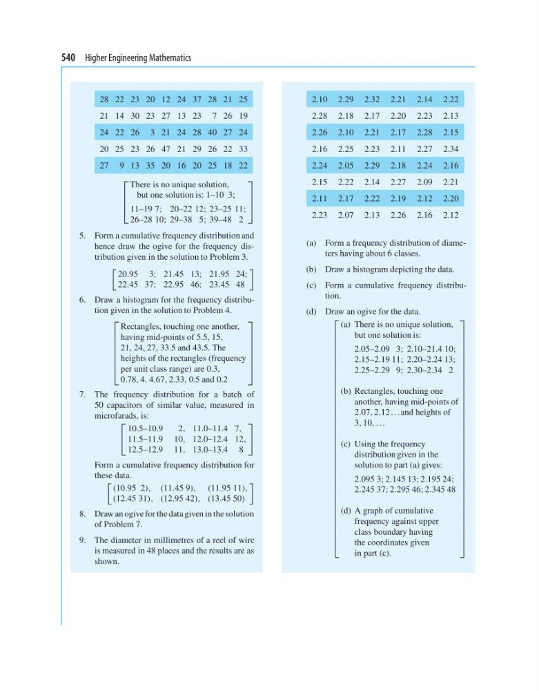
28 22 23 20 12 24 37 28 21 25
21 14 30 23 27 13 23 7 26 19
24 22 26 3 21 24 28 40 27 24
20 25 23 26 47 21 29 26 22 33
27 9 13 35 20 16 20 25 18 22
⎡
⎢
⎢
⎣
There is no unique solution,
but one solution is: 1–10 3;
11–19 7; 20–22 12; 23–25 11;
26–28 10; 29–38 5; 39–48 2
⎤
⎥
⎥
⎦
5. Form a cumulative frequency distribution and
hence draw the ogive for the frequency distribution given in the solution to Problem 3.
20.95 3; 21.45 13; 21.95 24;
22.45 37; 22.95 46; 23.45 48
6. Draw a histogram for the frequency distribution given in the solution to Problem 4.
⎡
⎢
⎢
⎢
⎢
⎢
⎢
⎣
Rectangles, touching one another,
having mid-points of 5.5, 15,
21, 24, 27, 33.5 and 43.5. The
heights of the rectangles (frequency
per unit class range) are 0.3,
0.78, 4. 4.67, 2.33, 0.5 and 0.2
⎤
⎥
⎥
⎥
⎥
⎥
⎥
⎦
7. The frequency distribution for a batch of
50 capacitors of similar value, measured in
microfarads, is:
⎡
⎣
10.5–10.9
2, 11.0–11.4 7,
11.5–11.9 10, 12.0–12.4 12,
12.5–12.9 11, 13.0–13.4 8
⎤
⎦
Form a cumulative frequency distribution for
these data.
(10.95 2), (11.45 9), (11.95 11),
(12.45 31), (12.95 42), (13.45 50)
8. Draw an ogive for the data given in the solution
of Problem 7.
9. The diameter in millimetres of a reel of wire
is measured in 48 places and the results are as
shown.
2.10 2.29 2.32 2.21 2.14 2.22
2.28 2.18 2.17 2.20 2.23 2.13
2.26 2.10 2.21 2.17 2.28 2.15
2.16 2.25 2.23 2.11 2.27 2.34
2.24 2.05 2.29 2.18 2.24 2.16
2.15 2.22 2.14 2.27 2.09 2.21
2.11 2.17 2.22 2.19 2.12 2.20
2.23 2.07 2.13 2.26 2.16 2.12
(a) Form a frequency distribution of diameters having about 6 classes.
(b) Draw a histogram depicting the data.
(c) Form a cumulative frequency distribution.
(d) Draw an ogive for the data.
⎡
⎢
⎢
⎢
⎢
⎢
⎢
⎢
⎢
⎢
⎢
⎢
⎢
⎢
⎢
⎢
⎢
⎢
⎢
⎢
⎢
⎢
⎢
⎢
⎢
⎢
⎢
⎢
⎢
⎢
⎢
⎢
⎢
⎢
⎢
⎢
⎢
⎢
⎢
⎢
⎣
(a) There is no unique solution,
but one solution is:
2.05–2.09 3; 2.10–21.4 10;
2.15–2.19 11; 2.20–2.24 13;
2.25–2.29 9; 2.30–2.34 2
(b) Rectangles, touching one
another, having mid-points of
2.07, 2.12 ...and heights of
3, 10, ...
(c) Using the frequency
distribution given in the
solution to part (a) gives:
2.095 3; 2.145 13; 2.195 24;
2.245 37; 2.295 46; 2.345 48
(d) A graph of cumulative
frequency against upper
class boundary having
the coordinates given
in part (c).
⎤
⎥
⎥
⎥
⎥
⎥
⎥
⎥
⎥
⎥
⎥
⎥
⎥
⎥
⎥
⎥
⎥
⎥
⎥
⎥
⎥
⎥
⎥
⎥
⎥
⎥
⎥
⎥
⎥
⎥
⎥
⎥
⎥
⎥
⎥
⎥
⎥
⎥
⎥
⎥
⎦
28 22 23 20 12 24 37 28 21 25
21 14 30 23 27 13 23 7 26 19
24 22 26 3 21 24 28 40 27 24
20 25 23 26 47 21 29 26 22 33
27 9 13 35 20 16 20 25 18 22
⎡
⎢
⎢
⎣
There is no unique solution,
but one solution is: 1–10 3;
11–19 7; 20–22 12; 23–25 11;
26–28 10; 29–38 5; 39–48 2
⎤
⎥
⎥
⎦
5. Form a cumulative frequency distribution and
hence draw the ogive for the frequency distribution given in the solution to Problem 3.
20.95 3; 21.45 13; 21.95 24;
22.45 37; 22.95 46; 23.45 48
6. Draw a histogram for the frequency distribution given in the solution to Problem 4.
⎡
⎢
⎢
⎢
⎢
⎢
⎢
⎣
Rectangles, touching one another,
having mid-points of 5.5, 15,
21, 24, 27, 33.5 and 43.5. The
heights of the rectangles (frequency
per unit class range) are 0.3,
0.78, 4. 4.67, 2.33, 0.5 and 0.2
⎤
⎥
⎥
⎥
⎥
⎥
⎥
⎦
7. The frequency distribution for a batch of
50 capacitors of similar value, measured in
microfarads, is:
⎡
⎣
10.5–10.9
2, 11.0–11.4 7,
11.5–11.9 10, 12.0–12.4 12,
12.5–12.9 11, 13.0–13.4 8
⎤
⎦
Form a cumulative frequency distribution for
these data.
(10.95 2), (11.45 9), (11.95 11),
(12.45 31), (12.95 42), (13.45 50)
8. Draw an ogive for the data given in the solution
of Problem 7.
9. The diameter in millimetres of a reel of wire
is measured in 48 places and the results are as
shown.
2.10 2.29 2.32 2.21 2.14 2.22
2.28 2.18 2.17 2.20 2.23 2.13
2.26 2.10 2.21 2.17 2.28 2.15
2.16 2.25 2.23 2.11 2.27 2.34
2.24 2.05 2.29 2.18 2.24 2.16
2.15 2.22 2.14 2.27 2.09 2.21
2.11 2.17 2.22 2.19 2.12 2.20
2.23 2.07 2.13 2.26 2.16 2.12
(a) Form a frequency distribution of diameters having about 6 classes.
(b) Draw a histogram depicting the data.
(c) Form a cumulative frequency distribution.
(d) Draw an ogive for the data.
⎡
⎢
⎢
⎢
⎢
⎢
⎢
⎢
⎢
⎢
⎢
⎢
⎢
⎢
⎢
⎢
⎢
⎢
⎢
⎢
⎢
⎢
⎢
⎢
⎢
⎢
⎢
⎢
⎢
⎢
⎢
⎢
⎢
⎢
⎢
⎢
⎢
⎢
⎢
⎢
⎣
(a) There is no unique solution,
but one solution is:
2.05–2.09 3; 2.10–21.4 10;
2.15–2.19 11; 2.20–2.24 13;
2.25–2.29 9; 2.30–2.34 2
(b) Rectangles, touching one
another, having mid-points of
2.07, 2.12 ...and heights of
3, 10, ...
(c) Using the frequency
distribution given in the
solution to part (a) gives:
2.095 3; 2.145 13; 2.195 24;
2.245 37; 2.295 46; 2.345 48
(d) A graph of cumulative
frequency against upper
class boundary having
the coordinates given
in part (c).
⎤
⎥
⎥
⎥
⎥
⎥
⎥
⎥
⎥
⎥
⎥
⎥
⎥
⎥
⎥
⎥
⎥
⎥
⎥
⎥
⎥
⎥
⎥
⎥
⎥
⎥
⎥
⎥
⎥
⎥
⎥
⎥
⎥
⎥
⎥
⎥
⎥
⎥
⎥
⎥
⎦