

538 Higher Engineering Mathematics
to the appropriate class by putting a ‘1’ in the appropriate row. Each fifth ‘1’ allocated to a particular row is
marked as an oblique line to help with final counting.
A frequency distribution for the data is shown in
Table 54.5 and lists classes and their corresponding frequencies. Class mid-points are also shown in this table,
since they are used when constructing the frequency
polygon and histogram.
Table 54.5
Class
Class mid-point Frequency
7.1 to 7.3
7.2
3
7.4 to 7.6
7.5
5
7.5 to 7.9
7.8
9
8.0 to 8.2
8.1
14
8.1 to 8.5
8.4
11
8.2 to 8.8
8.7
6
8.9 to 9.1
9.0
2
A frequency polygon is shown in Fig. 54.9, the
co-ordinates corresponding to the class midpoint/frequency values, given in Table 54.5. The
co-ordinates are joined by straight lines and the polygon is ‘anchored-down’ at each end by joining to the
next class mid-point value and zero frequency.
7.2
4
2
0
6
Frequency
12
10
8
14
7.8
7.5
8.1
Class mid-point values
8.7
9.0
8.4
Frequency polygon
Figure 54.9
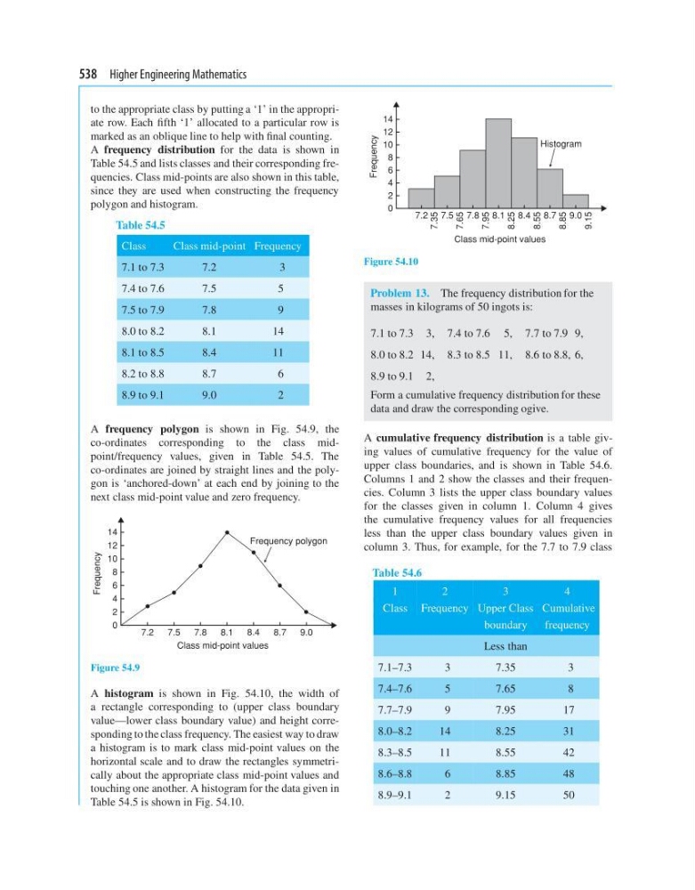
A histogram is shown in Fig. 54.10, the width of
a rectangle corresponding to (upper class boundary
value—lower class boundary value) and height corresponding to the class frequency. The easiest way to draw
a histogram is to mark class mid-point values on the
horizontal scale and to draw the rectangles symmetrically about the appropriate class mid-point values and
touching one another. A histogram for the data given in
Table 54.5 is shown in Fig. 54.10.
7.2
4
2
0
6
Frequency
10
8
12
14
7.5
7.35
7.65
7.95
8.25
8.55
8.85
9.15
7.8 8.1 8.4
Class mid-point values
9.0
8.7
Histogram
Figure 54.10
Problem 13. The frequency distribution for the
masses in kilograms of 50 ingots is:
7.1 to 7.3 3, 7.4 to 7.6 5, 7.7 to 7.9 9,
8.0 to 8.2 14, 8.3 to 8.5 11, 8.6 to 8.8, 6,
8.9 to 9.1 2,
Form a cumulative frequency distribution for these
data and draw the corresponding ogive.
A cumulative frequency distribution is a table giving values of cumulative frequency for the value of
upper class boundaries, and is shown in Table 54.6.
Columns 1 and 2 show the classes and their frequencies. Column 3 lists the upper class boundary values
for the classes given in column 1. Column 4 gives
the cumulative frequency values for all frequencies
less than the upper class boundary values given in
column 3. Thus, for example, for the 7.7 to 7.9 class
Table 54.6
1
2
3
4
Class Frequency Upper Class Cumulative
boundary
frequency
Less than
7.1–7.3
3
7.35
3
7.4–7.6
5
7.65
8
7.7–7.9
9
7.95
17
8.0–8.2
14
8.25
31
8.3–8.5
11
8.55
42
8.6–8.8
6
8.85
48
8.9–9.1
2
9.15
50
to the appropriate class by putting a ‘1’ in the appropriate row. Each fifth ‘1’ allocated to a particular row is
marked as an oblique line to help with final counting.
A frequency distribution for the data is shown in
Table 54.5 and lists classes and their corresponding frequencies. Class mid-points are also shown in this table,
since they are used when constructing the frequency
polygon and histogram.
Table 54.5
Class
Class mid-point Frequency
7.1 to 7.3
7.2
3
7.4 to 7.6
7.5
5
7.5 to 7.9
7.8
9
8.0 to 8.2
8.1
14
8.1 to 8.5
8.4
11
8.2 to 8.8
8.7
6
8.9 to 9.1
9.0
2
A frequency polygon is shown in Fig. 54.9, the
co-ordinates corresponding to the class midpoint/frequency values, given in Table 54.5. The
co-ordinates are joined by straight lines and the polygon is ‘anchored-down’ at each end by joining to the
next class mid-point value and zero frequency.
7.2
4
2
0
6
Frequency
12
10
8
14
7.8
7.5
8.1
Class mid-point values
8.7
9.0
8.4
Frequency polygon
Figure 54.9
A histogram is shown in Fig. 54.10, the width of
a rectangle corresponding to (upper class boundary
value—lower class boundary value) and height corresponding to the class frequency. The easiest way to draw
a histogram is to mark class mid-point values on the
horizontal scale and to draw the rectangles symmetrically about the appropriate class mid-point values and
touching one another. A histogram for the data given in
Table 54.5 is shown in Fig. 54.10.
7.2
4
2
0
6
Frequency
10
8
12
14
7.5
7.35
7.65
7.95
8.25
8.55
8.85
9.15
7.8 8.1 8.4
Class mid-point values
9.0
8.7
Histogram
Figure 54.10
Problem 13. The frequency distribution for the
masses in kilograms of 50 ingots is:
7.1 to 7.3 3, 7.4 to 7.6 5, 7.7 to 7.9 9,
8.0 to 8.2 14, 8.3 to 8.5 11, 8.6 to 8.8, 6,
8.9 to 9.1 2,
Form a cumulative frequency distribution for these
data and draw the corresponding ogive.
A cumulative frequency distribution is a table giving values of cumulative frequency for the value of
upper class boundaries, and is shown in Table 54.6.
Columns 1 and 2 show the classes and their frequencies. Column 3 lists the upper class boundary values
for the classes given in column 1. Column 4 gives
the cumulative frequency values for all frequencies
less than the upper class boundary values given in
column 3. Thus, for example, for the 7.7 to 7.9 class
Table 54.6
1
2
3
4
Class Frequency Upper Class Cumulative
boundary
frequency
Less than
7.1–7.3
3
7.35
3
7.4–7.6
5
7.65
8
7.7–7.9
9
7.95
17
8.0–8.2
14
8.25
31
8.3–8.5
11
8.55
42
8.6–8.8
6
8.85
48
8.9–9.1
2
9.15
50